Lecture 07: Distance & acceleration

PHYS 351 · Lecture 0701

Lecture 07

Ultrasonic Range Finding and Three-Axis Accelerometry

Covers Lab 7

PHYS 351 · Lecture 0702

Today, in one line

The sensor measures. You convert.

A time becomes a distance only if you know the speed of sound.

An acceleration becomes an angle only if you know gravity is always there.

Every assumption is an error you can size.

PHYS 351 · Lecture 0703

Where each task points

Task	You do	Idea
1	HC-SR04 script and schematic; build; approval; m, cm, mm, inches	time of flight, 5 V Echo
2	zero offset, min and max range, accuracy; vs datasheet	calibration
3	LIS3DH wired; find its address; validate the $x$ axis	I²C again
4	100+ points per axis; $\sigma$ at rest; tilt theory; smallest angle	gravity, noise
5	average $n$ readings; $\sigma$ of averages; plot; CSV	$\sigma/\sqrt{n}$
6	pendulum, three axes, 10 s+; plot; explain the frequencies	$f$ and $2f$
7	add the MCP9808; temperature-compensated distance	speed of sound vs $T$

PHYS 351 · Lecture 0704

Time of flight

PHYS 351 · Lecture 0705

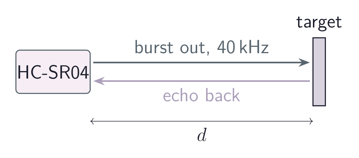
There and back

Ultrasonic distance measurement: the sensor sends a pulse toward a target and receives its reflected echo. Sound travels the distance twice, so distance equals sound speed times elapsed time divided by two.

d = \frac{v_{\text{sound}}\,t}{2}

Forget the 2 and every reading is exactly double, and self-consistent. Check one distance with a ruler.

PHYS 351 · Lecture 0706

A number worth memorising

At about $20\degC$ : $v \approx 343$ m/s $= 34.3$ cm per ms.

1\ \text{cm of distance} \;\rightarrow\; 2\ \text{cm of travel} \;\rightarrow\; \approx 58\us

10 cm target $\rightarrow$ ? 2 m target $\rightarrow$ ?

PHYS 351 · Lecture 0707

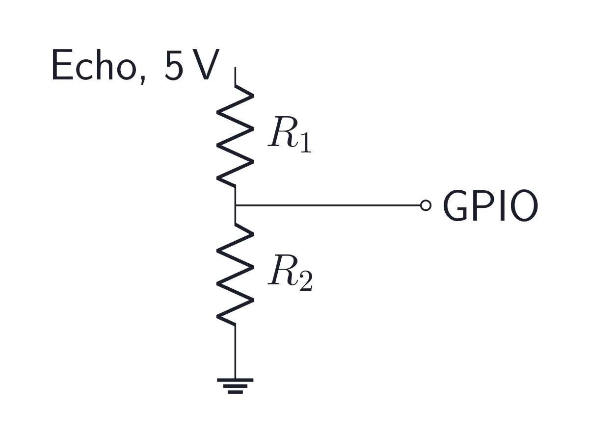
HC-SR04: four pins, one hazard

Pin	Note
VCC	5 V; 3.3 V is not reliable
Trig	Pi $\rightarrow$ module; 10 $\upmu$ s pulse; 3.3 V is enough
Echo	module $\rightarrow$ Pi; 5 V high level
GND	shared

V_{\text{GPIO}} = V_{\text{Echo}}\,\frac{R_2}{R_1+R_2}

HC-SR04 Echo voltage divider: the 5 V Echo output feeds a resistor divider, and its midpoint feeds a Raspberry Pi GPIO input. The lower resistor returns to common ground, reducing the input voltage to a safe level.

Never Echo straight to a pin

Divide 5 V to well below 3.3 V. Measure the node before connecting it.

PHYS 351 · Lecture 0708

The measurement sequence

1. Trig high for about 10 $\upmu$ s, then low.

2. Echo goes high.

3. Echo goes low when the echo returns. Its width is $t$ .

Time it with time.perf_counter(): rise, fall, subtract.

Always a timeout

No echo, and a naive while waits forever. Decide what “no reading” looks like.

PHYS 351 · Lecture 0709

Lecture 03 comes back with teeth

\Delta d = \frac{v\,\Delta t}{2} \approx 0.017\ \text{cm per}\ \upmu\text{s}

Python catches an edge to maybe 100 $\upmu$ s: $\Delta d \approx 1.7$ cm.

The datasheet’s 3 mm is out of reach this way. Knowing why is the point.

Measure your own scatter: fixed target, 100 readings, standard deviation.

PHYS 351 · Lecture 0710

Significant figures (Task 1e)

Unit conversion invents precision.

Good to a centimetre, yet 0.4372 m, 43.72 cm, 437.2 mm, 17.21 in all claim a tenth of a millimetre.

Decide the real uncertainty first. Same physical precision in every unit.

PHYS 351 · Lecture 0711

Calibrating the range finder (Task 2)

Quantity	Meaning	Method
Zero offset	constant reported minus true	known distances; fit a line; the intercept
Minimum range	echo returns before the module listens	bring a flat target closer until readings stop tracking
Maximum range	echo too weak	large flat target, move it away; say what target
Accuracy	repeatability and trueness	$\sigma$ of 100 readings; mean vs ruler. Two numbers.

Contaminants: target angle, soft material, a $15^\circ$ beam, stray echoes.

PHYS 351 · Lecture 0712

Temperature compensation (Task 7)

v_{\text{sound}} \approx 331.3 + 0.606\,T\quad \text{m/s},\ T\ \text{in}\ \degC

$0\degC$ : 331.3. $30\degC$ : 349.5. 5.5 % in speed is 5.5 % in distance: 11 cm at 2 m.

Far above the timing floor. The thermometer removes the dominant error.

Show it: log both for one target, then warm the sensor.

PHYS 351 · Lecture 0713

The accelerometer

PHYS 351 · Lecture 0714

At rest it does not read zero

A proof mass on springs measures proper acceleration: relative to free fall.

On the bench: 1 g on the vertical axis, 0 on the others.

In free fall: 0 on all three. “Zero g” means falling.

The basis of measuring tilt.

PHYS 351 · Lecture 0715

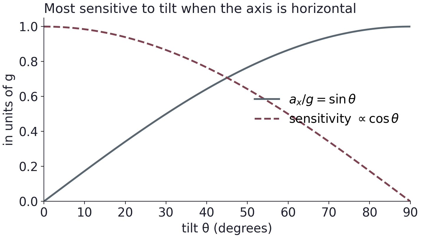
Tilt from gravity

Accelerometer tilt response ax/g equals sine theta, while angular sensitivity is proportional to cosine theta. Sensitivity is greatest near a horizontal axis and tends to zero near 90 degrees.

a_x = g\sin\theta

\frac{\mathrm{d}a_x}{\mathrm{d}\theta} = g\cos\theta

Flat: very sensitive to a small tip.

On end: almost blind to it.

PHYS 351 · Lecture 0716

The LIS3DH: same architecture

Sensing element, ADC, registers, I²C. Lecture 06 applies.

i2cdetect -y 1: read the address off the scan
read the ID register first
smallest full-scale range; widen only if you see flat tops
two’s complement: the sign bug hides while readings are positive

PHYS 351 · Lecture 0717

Validate the axes for free (Task 3)

Gravity is a stable 1 g reference that is always available.

Flat: $+1$ g. Upside down: $-1$ g. On each edge: 1 g moves to the right axis with the right sign.

Six orientations check every axis, both signs, the scale factor, and which label points where.

PHYS 351 · Lecture 0718

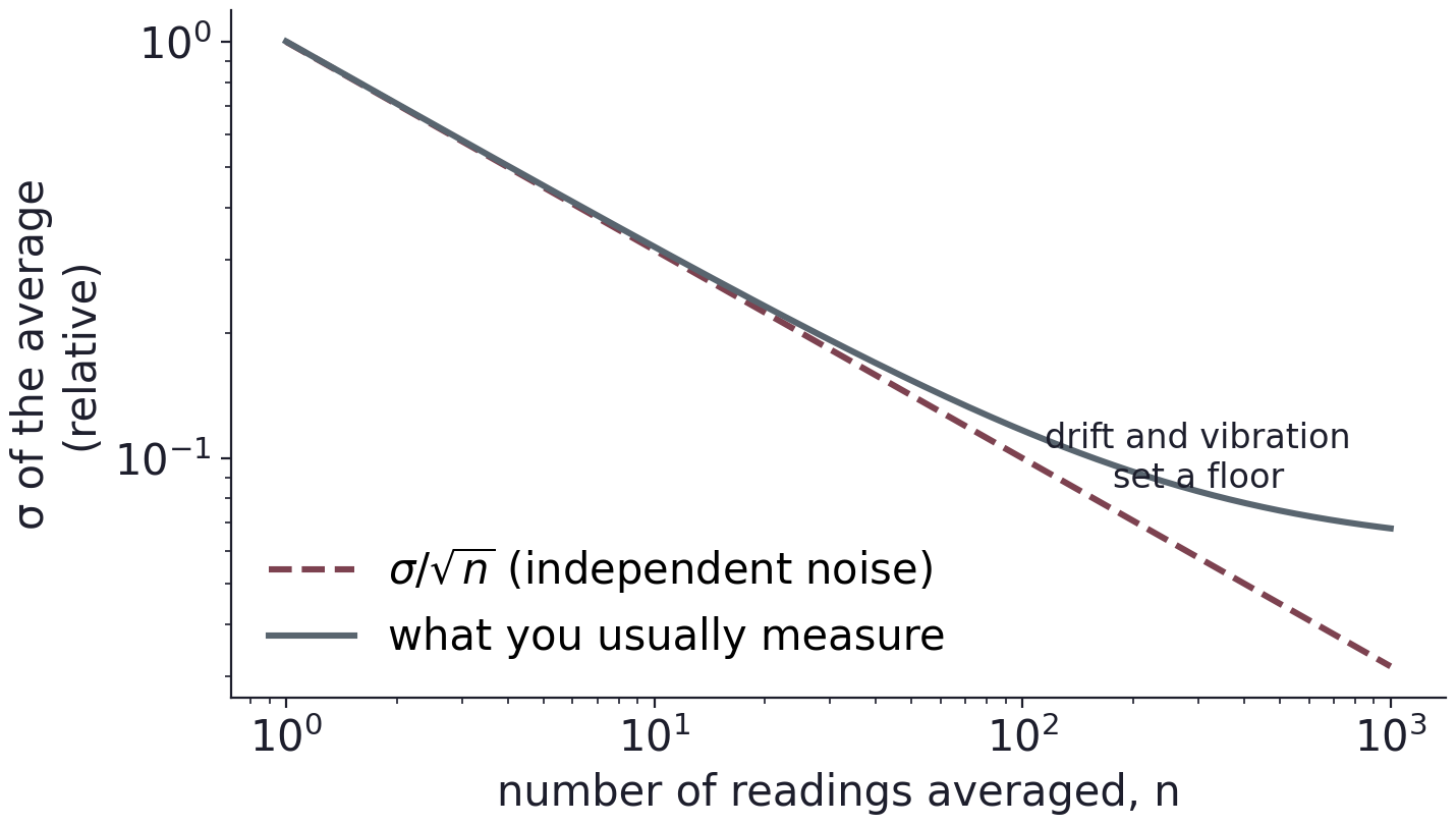
Noise floor and averaging (Tasks 4, 5)

Log-log sketch of uncertainty versus number of averaged readings. Independent noise decreases as one over the square root of n, but measured uncertainty eventually approaches a drift and vibration floor.

\sigma_{\text{mean}} = \frac{\sigma}{\sqrt{n}}

Independent noise only.

Drift and vibration are correlated: the curve flattens. Where, is a result.

PHYS 351 · Lecture 0719

Smallest detectable tilt

\Delta\theta = \frac{\Delta a}{g\cos\theta}

$\Delta a$ is your noise floor, or $2\sigma$ for a confident detection. State the criterion and $\theta$ .

$\sigma = 0.004$ g, horizontal, $2\sigma$ criterion: $\Delta\theta$ = ?

PHYS 351 · Lecture 0720

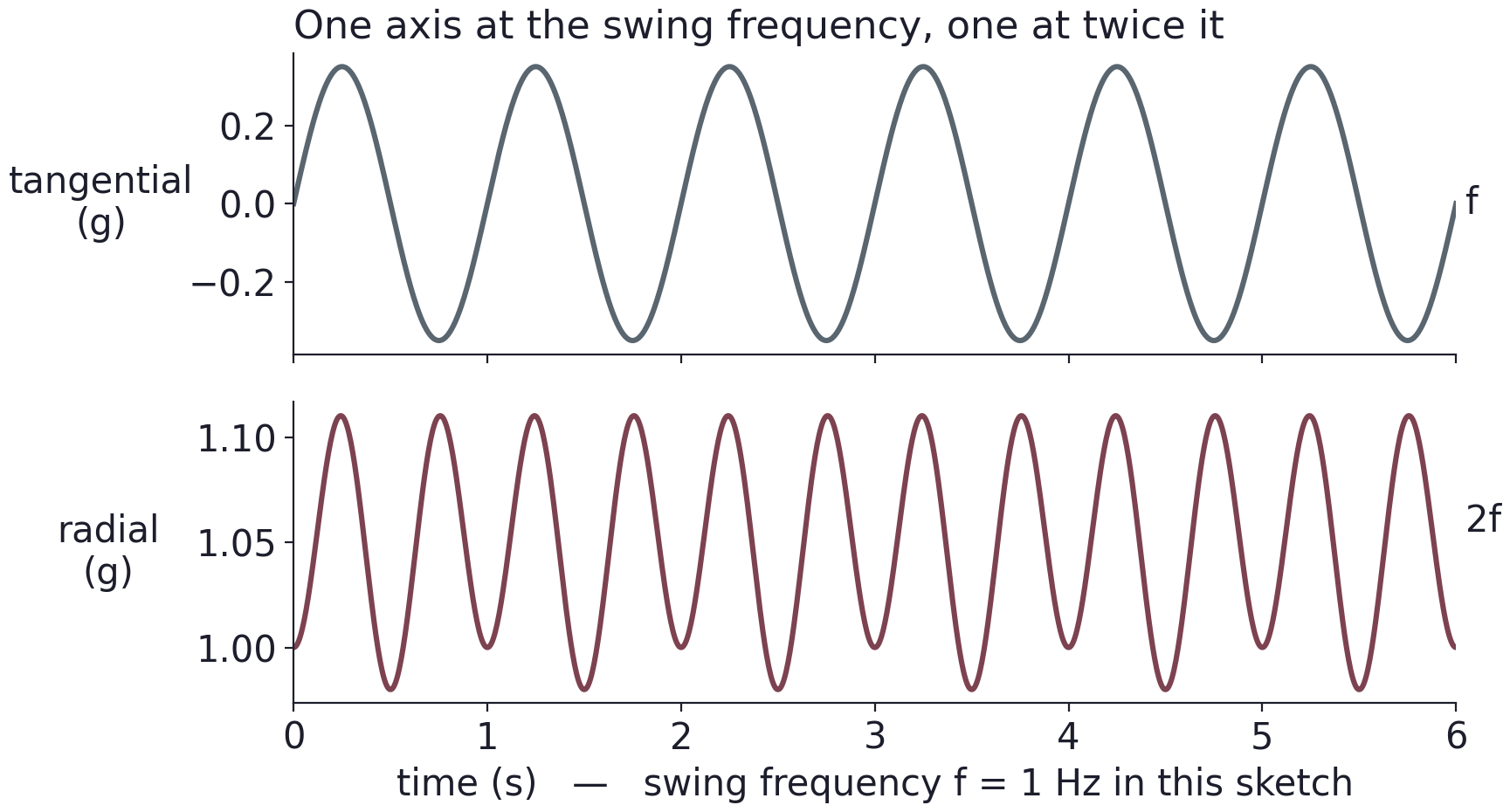
The pendulum (Task 6)

Conceptual pendulum signals: tangential acceleration oscillates at the swing frequency f; radial acceleration oscillates at twice that frequency, 2f, about a gravity offset.

f_{\text{swing}} = \frac{1}{2\pi}\sqrt{\frac{g}{L}}

Tangential $\propto \sin\theta$ : $f$ .

Radial $= v^2/L$ : positive, peaks at the bottom, twice per swing: $2f$ .

PHYS 351 · Lecture 0721

Data worth analysing

know which axis is radial and which tangential before you swing
sample at tens of Hz: you must resolve $2f$
one plane, modest amplitude
$L$ is pivot to centre of mass
the cable adds stiffness and damping; say how you managed it

PHYS 351 · Lecture 0722

Destroys hardware / wastes your afternoon

Destroys hardware

Echo straight to a GPIO pin
5 V to the LIS3DH
VCC and GND swapped
wiring a live bus

Wastes your afternoon

the missing factor of two
no timeout on Echo
max range against a curtain
expecting 0 g at rest
two’s complement sign bug
sampling too slowly for $2f$

Light bob, modest swing, pivot secured, arc clear.

PHYS 351 · Lecture 0723

Take away

A range finder measures time, so your timing precision is your distance precision, and the speed of sound is a bigger error than your code unless you measure the temperature.

An accelerometer measures proper acceleration: 1 g at rest, zero in free fall, and gravity becomes a free reference for calibration and tilt.

PHYS 351 · Lecture 0724

Exit check

1. Echo pulse 2.90 ms wide at $20\degC$ : distance in cm?

2. Edge timing uncertain by 60 $\upmu$ s: distance uncertainty?

3. Speed of sound change from 15 to $30\degC$ , and the error at 1.5 m?

4. Pendulum at 1.2 Hz: tangential axis frequency? Radial?

Use ← → to move, Home / End to jump, and F for fullscreen.

Figure descriptions

Slide 5 · There and back

Ultrasonic distance measurement: the sensor sends a pulse toward a target and receives its reflected echo. Sound travels the distance twice, so distance equals sound speed times elapsed time divided by two.

Slide 7 · HC-SR04: four pins, one hazard

HC-SR04 Echo voltage divider: the 5 V Echo output feeds a resistor divider, and its midpoint feeds a Raspberry Pi GPIO input. The lower resistor returns to common ground, reducing the input voltage to a safe level.

Slide 15 · Tilt from gravity

Accelerometer tilt response ax/g equals sine theta, while angular sensitivity is proportional to cosine theta. Sensitivity is greatest near a horizontal axis and tends to zero near 90 degrees.

Slide 18 · Noise floor and averaging (Tasks 4, 5)

Slide 20 · The pendulum (Task 6)

Conceptual pendulum signals: tangential acceleration oscillates at the swing frequency f; radial acceleration oscillates at twice that frequency, 2f, about a gravity offset.