Lecture 08: ADC, SPI & remote access

PHYS 351 · Lecture 0801

Lecture 08

SPI, the MCP3008 ADC, and Remote Access

Covers Lab 8

PHYS 351 · Lecture 0802

Today, in one line

An ADC replaces a continuous voltage with a number from a finite set, at particular instants.

Quantisation sets how finely you resolve a value.

Sampling rate sets which frequencies you can believe.

PHYS 351 · Lecture 0803

Where each task points

Task	You do	Idea
1	network, directory, OS update, enable SPI, download the module	bringing SPI up
2	wire the MCP3008; read a channel as volts; demonstrate	wiring, counts to volts
3	a 0–3.3 V source; compare with the DMM; error handling	calibration budget
4	raw counts and volts, 20+ points; plot; linearity	the transfer function
5	sine into ADC and scope; plot $V(t)$ ; maximum usable frequency	sampling, Nyquist, aliasing
6–7	SSH from a laptop; VNC desktop; run programs remotely	remote access

The one lab that needs the internet: plan time for the OS update.

PHYS 351 · Lecture 0804

The SPI bus

PHYS 351 · Lecture 0805

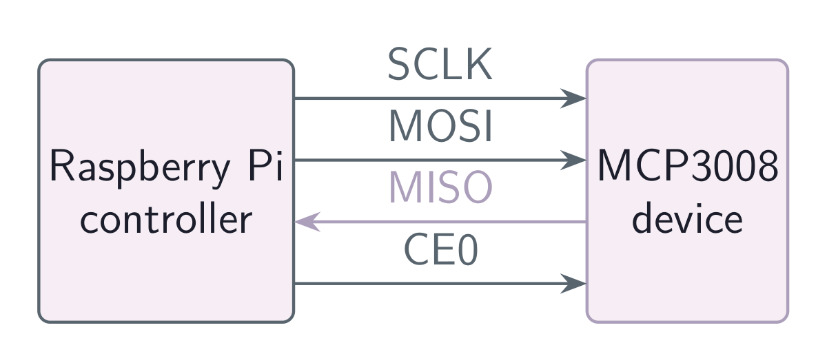
Four wires

SPI signal directions between Raspberry Pi controller and MCP3008 device: SCLK and MOSI travel from controller to ADC, MISO returns data to the controller, and CE0 selects the ADC. Power and ground connections are not drawn.

Signal	Direction	Pi pin
SCLK	clock, Pi $\rightarrow$	BCM 11, phys 23
MOSI	data, Pi $\rightarrow$	BCM 10, phys 19
MISO	data, $\rightarrow$ Pi	BCM 9, phys 21
CE0	chip select	BCM 8, phys 24

Clock and data are shared. Only the select line is per device.

PHYS 351 · Lecture 0806

A shift register spanning two chips

Select goes low. Each clock moves one bit out on MOSI and one bit in on MISO, at the same time.

Full duplex, and it matters here

To receive a byte you must send a byte. Reading the MCP3008 is one three-byte swap.

No addresses, no acknowledge, no START or STOP. Simpler, and much faster.

PHYS 351 · Lecture 0807

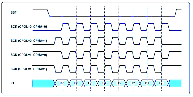
Clock polarity and phase

Mode	CPOL	CPHA	Latches
0	0	0	rising edge
1	0	1	falling edge
2	1	0	falling edge
3	1	1	rising edge

MCP3008: mode 0, the default.

Data shifted one bit: mode mismatch.

PHYS 351 · Lecture 0808

SPI against I²C

	I²C (Labs 6, 7)	SPI (Lab 8)
Wires	2, whatever the device count	3 shared + 1 select per device
Selection	7-bit address on the bus	a dedicated pin
Speed	100–400 kHz	several MHz
Direction	half duplex	full duplex
Electrical	open drain, pull-ups, active low	push–pull
Errors	ACK/NAK on every byte	none
Discovery	`i2cdetect`	none at all

I²C spends speed to save pins. SPI spends pins to buy speed.

PHYS 351 · Lecture 0809

Bringing SPI up

sudo raspi-config     # Interface Options -> SPI -> Yes; reboot
ls /dev/spidev*       # expect spidev0.0 and spidev0.1

There is no spidetect. A mis-wired chip returns zeros or plausible nonsense, not an error.

The known-input tests near the end of this deck are the substitute.

PHYS 351 · Lecture 0810

What an ADC does

PHYS 351 · Lecture 0811

Two approximations, kept separate

Sampling discretises time. Which frequencies you can represent.

Quantisation discretises amplitude. How precisely you resolve a value.

Neither can be fixed afterwards in software.

PHYS 351 · Lecture 0812

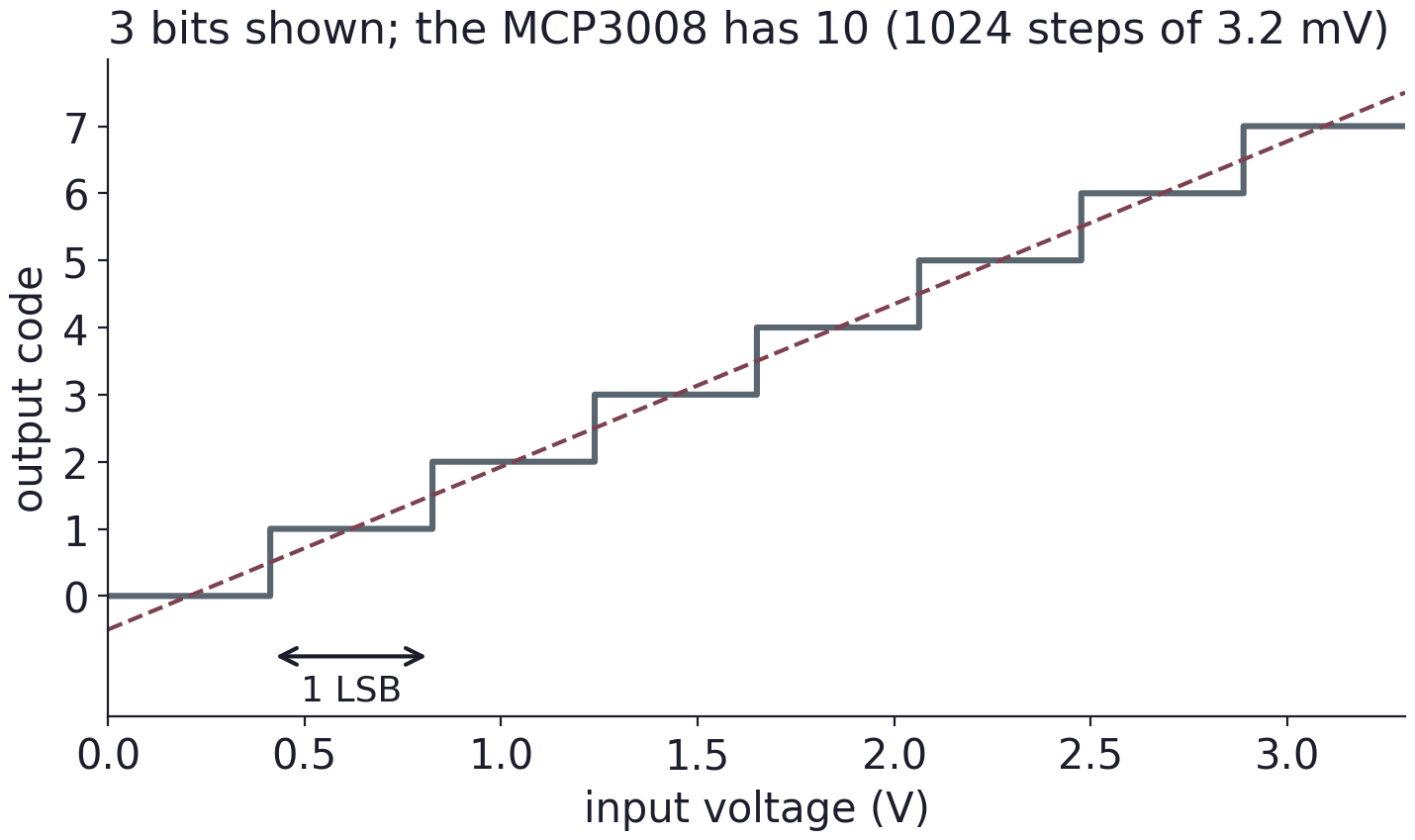
Quantisation and the LSB

ADC transfer staircase: analog input is mapped to discrete output codes. The sketch shows three bits; the MCP3008 uses ten bits, giving 1024 levels and about 3.2 mV per level for a 3.3 V reference.

V_{\text{LSB}} = \frac{V_{\text{ref}}}{2^N}

10 bits, 3.3 V: $3.3/1024 = 3.22$ mV.

Any single reading: $\pm\tfrac12$ LSB, about $\pm 1.6$ mV.

PHYS 351 · Lecture 0813

1024 levels, counts 0 to 1023

There is no count of 1024. Same off-by-one as an array of length 1024.

V = \frac{\text{count}}{1023}\,V_{\text{ref}} \qquad\text{or}\qquad V = \frac{\text{count}}{1024}\,V_{\text{ref}}

Pick one, state it, use it everywhere. They differ by about 3 mV at full scale: the size of effect Task 3 measures.

PHYS 351 · Lecture 0814

Successive approximation

A binary search inside the chip. Upper half or lower half? That is the MSB.

Halve the interval, compare again, next bit. Ten comparisons, ten bits.

Conversion time grows with resolution: the MCP9808’s trade again.

PHYS 351 · Lecture 0815

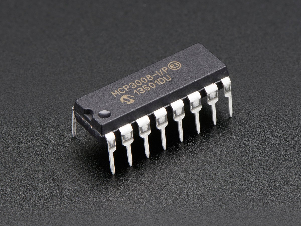
The MCP3008

MCP3008 analog-to-digital converter in a 16-pin dual-inline package, showing its identifying label and orientation notch. Photo: Adafruit.
10 bits, 8 channels, one converter shared

Pin	Connect to
VDD	3.3 V
VREF	3.3 V: sets the full-scale range
AGND, DGND	ground, both
CLK	BCM 11 (SCLK)
DIN	BCM 10 (MOSI)
DOUT	BCM 9 (MISO)
CS/SHDN	BCM 8 (CE0)
CH0–CH7	your signal, 0 V to VREF

Count pins from the notch.

PHYS 351 · Lecture 0816

Never exceed the input range

0 V to VREF, nothing else

A function generator’s sine swings about zero. The negative half can damage the chip.

Offset the signal so it sits entirely inside 0–3.3 V, with the generator’s DC offset.

Set amplitude and offset on the scope before the ADC sees it.

PHYS 351 · Lecture 0817

The volts-vs-counts plot (Task 4)

A straight line through the origin, and a test of the converter:

slope $\approx 3.2$ mV per count. Different? Your real VREF is not 3.300 V. Measure the rail.
intercept zero. Not? A ground or offset problem.
plot the residuals: $\pm\tfrac12$ LSB scatter, or a systematic curve

Output the raw count too: that is what the hardware produced.

PHYS 351 · Lecture 0818

Comparing with the DMM (Task 3): set the budget first

quantisation: $\pm 1.6$ mV, unavoidable
the DMM’s own accuracy specification
VREF is whatever the rail actually is
noise, which averaging shrinks

“Within 4 mV, consistent with quantisation plus the meter’s stated accuracy” is a result. “Close” is not.

PHYS 351 · Lecture 0819

Sampling

PHYS 351 · Lecture 0820

What sets your sampling rate

The ADC: hundreds of thousands of samples per second.

The SPI clock: three bytes per conversion at MHz.

Your Python loop: a call, an SPI transaction, an append, under Linux. This one binds.

Time a few thousand conversions with perf_counter(). Report the rate and its spread.

PHYS 351 · Lecture 0821

The sampling theorem

f_{\text{sample}} > 2 f_{\text{signal}} \qquad\Longleftrightarrow\qquad f_{\max} = \frac{f_{\text{sample}}}{2}

Half the sampling rate is the Nyquist frequency.

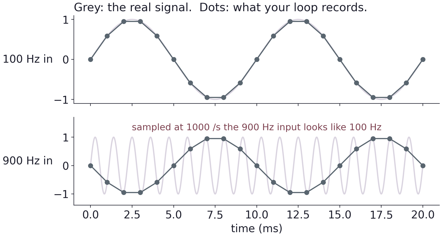
Above it information is not degraded. It is destroyed, and replaced by something that looks real.

PHYS 351 · Lecture 0822

Aliasing

Sampling at 1000 samples per second: a 100 Hz sine wave is resolved, while samples of a 900 Hz sine wave appear to follow a 100 Hz wave. Sample points alone cannot distinguish these frequencies. — The 900 Hz case is the dangerous one: nothing in the data looks wrong. The scope shows the truth.

PHYS 351 · Lecture 0823

Answering Task 5 properly

“Maximum frequency” needs a definition:

absolute limit: $f_{\text{sample}}/2$
practical limit for a recognisable shape: perhaps $f_{\text{sample}}/10$ ; define “recognisable”
jitter degrades things further as the period shrinks

A real instrument adds a low-pass first: the Lab 1 RC filter, as an anti-alias filter.

PHYS 351 · Lecture 0824

Remote access

PHYS 351 · Lecture 0825

SSH and VNC

Method	You get	Use it for
SSH	a terminal on the Pi, on your laptop	scripts, editing, anything command-line
VNC	the Pi’s whole desktop, mirrored	anything graphical; heavy on the network

hostname -I                       # on the Pi: its address
sudo raspi-config                 # Interface Options -> SSH, VNC
ssh pi@<address>                  # from your laptop
scp pi@<address>:lab8/data.csv .  # copy back

PHYS 351 · Lecture 0826

Why a plot needs more than SSH

SSH carries text. plt.show() has no display: it fails or hangs.

save the figure to a PNG and scp it back
VNC: a real desktop for the window (Task 7)
ssh -X: tunnel individual windows

Same network as the Pi; campus Wi-Fi often isolates clients. Change the default password.

PHYS 351 · Lecture 0827

Debugging SPI without a detect command

1. /dev/spidev0.0 exists? No: enable, reboot.

2. Ground the input: read $\approx 0$ ?

3. Input to 3.3 V: read $\approx$ full scale?

4. Always zero: MISO, chip select, or power.

5. Wildly fluctuating: a floating input. Normal.

6. Exactly half or double: a bit shift, or the SPI mode.

PHYS 351 · Lecture 0828

Destroys hardware / wastes your afternoon

Destroys hardware

input outside 0 to VREF
5 V to the chip or its inputs
VDD and ground swapped
rewiring with power on

Wastes your afternoon

MOSI and MISO confused
VREF left floating
assuming exactly 3.300 V
1023 and 1024 mixed
a sine with no offset
plotting inside the sampling loop

Before you leave: copy everything off, remove your directory.

PHYS 351 · Lecture 0829

Take away

An ADC turns a voltage into a number, and both axes of that conversion are approximations you can quantify.

Quantisation sets the finest voltage you can see. The sampling rate, set here by your loop and not the hardware, sets the highest frequency you can believe.

Sample too slowly and the signal does not disappear. It lies to you.

PHYS 351 · Lecture 0830

Exit check

1. LSB size for 10 bits at 3.3 V, and the error of a single reading?

2. 800 samples/s: highest faithful frequency? What does 750 Hz look like?

3. Three differences between SPI and I²C, and which suits which device?

4. Which two known inputs bracket the transfer function?

Use ← → to move, Home / End to jump, and F for fullscreen.

Figure descriptions

Slide 5 · Four wires

SPI signal directions between Raspberry Pi controller and MCP3008 device: SCLK and MOSI travel from controller to ADC, MISO returns data to the controller, and CE0 selects the ADC. Power and ground connections are not drawn.

Slide 7 · Clock polarity and phase

SPI timing for all four CPOL and CPHA combinations. Clock idle level and sampling edge change between modes, while chip select frames the byte transfer.

Slide 12 · Quantisation and the LSB