Part 1 · Lab 1 in five tasks
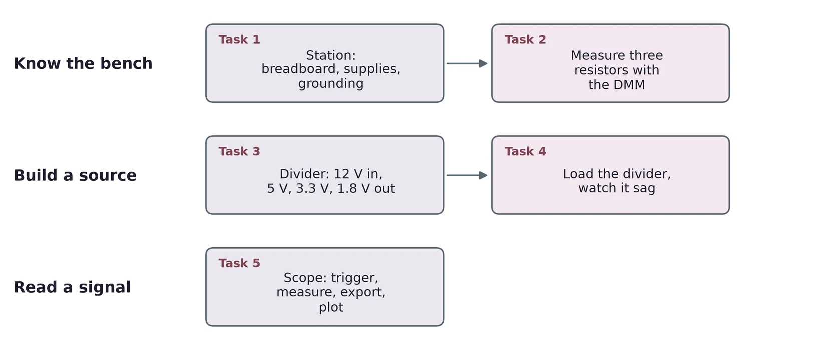
First you learn the bench and measure parts. Then you build a source from resistors and watch it sag under load. Last, you read a signal on the scope.
The breadboard joins holes in strips of five
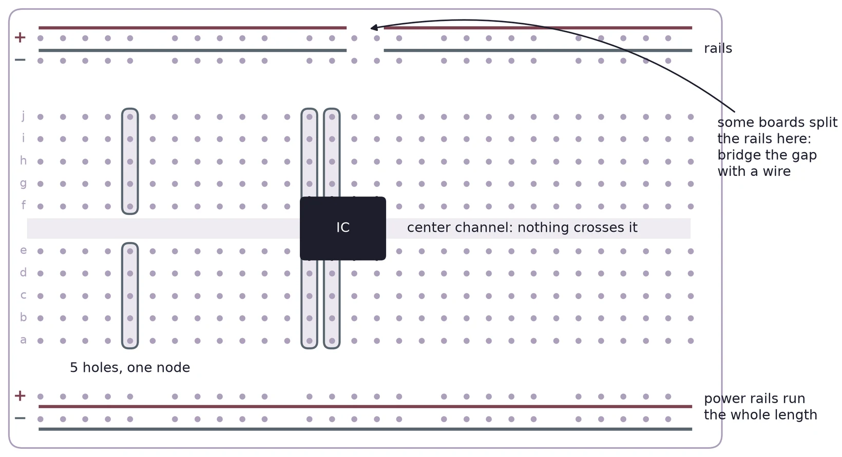
Each column of five holes is one node. Chips straddle the center channel, so each pin gets its own strip.
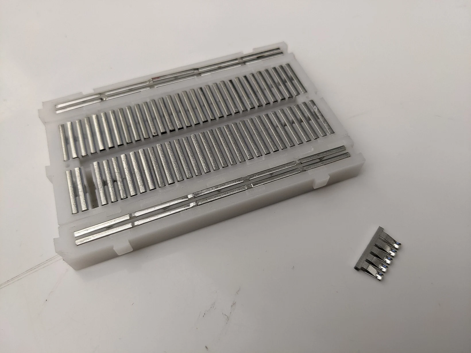
Inside: one spring clip per strip


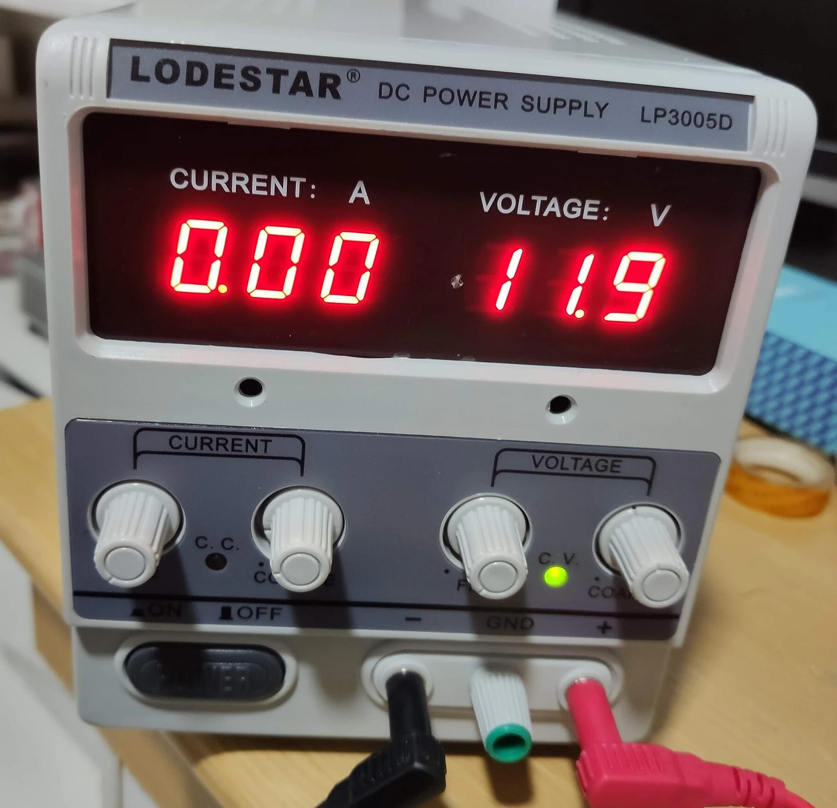
Two kinds of power supply
| Integrated | External | |
|---|---|---|
| Where | built into the station | separate box |
| Voltage | fixed or adjustable | adjustable |
| Current limit | internal fuse or limit | knob you set |
| Ground | shared with the station | floating until you connect it |
Set the current limit just above what your circuit needs. Photo: Derrick Parker, CC0.

The DMM: across for volts, in series for amps
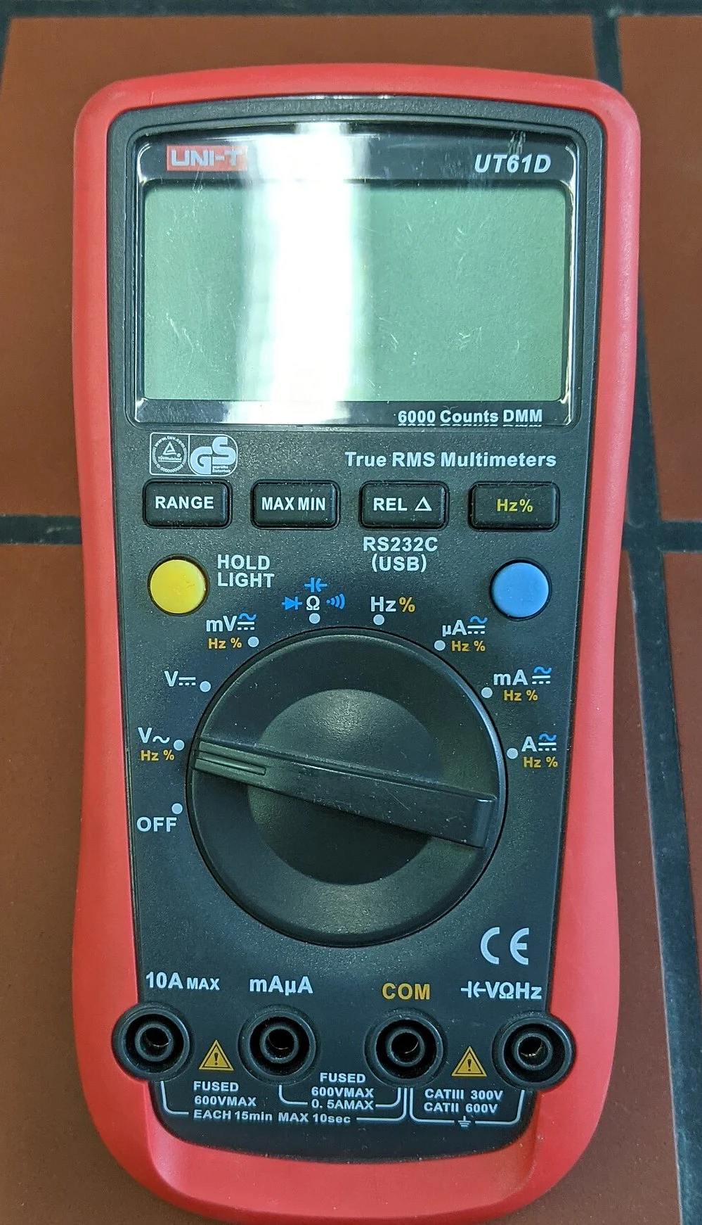
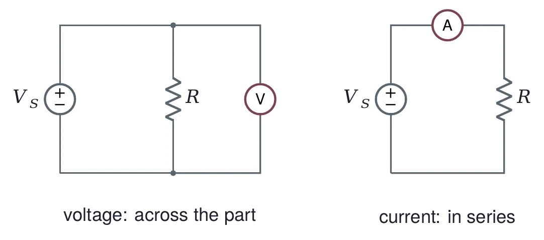
Resistance: take the part out of the circuit, power off.
Move the red lead to the A or mA jack only for current. Photo: Anselm Schüler, CC BY-SA 4.0.

Read the color code
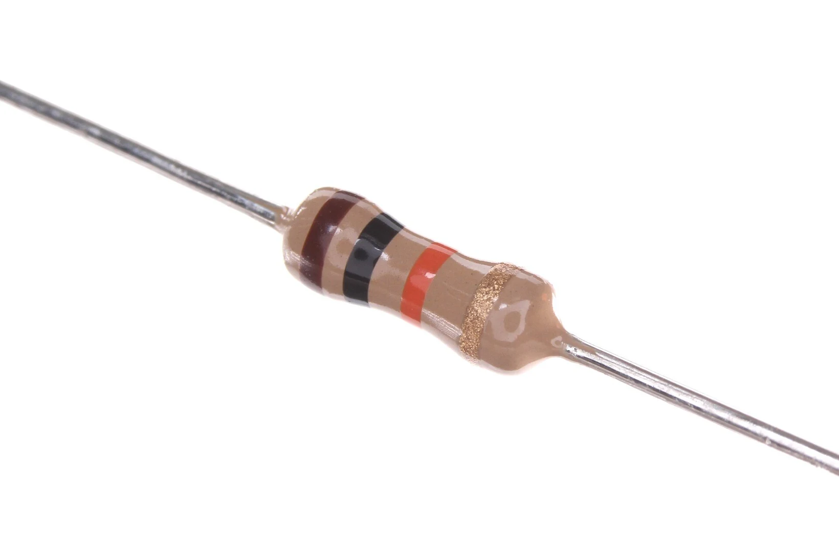
Brown, black, orange, gold: , ±5 %
| Color | Digit | Color | Digit |
|---|---|---|---|
| black | 0 | green | 5 |
| brown | 1 | blue | 6 |
| red | 2 | violet | 7 |
| orange | 3 | gray | 8 |
| yellow | 4 | white | 9 |
Tolerance: gold ±5 %, silver ±10 %, brown ±1 %
Photo: oomlout, CC BY-SA 2.0.

Standard values come in E-series
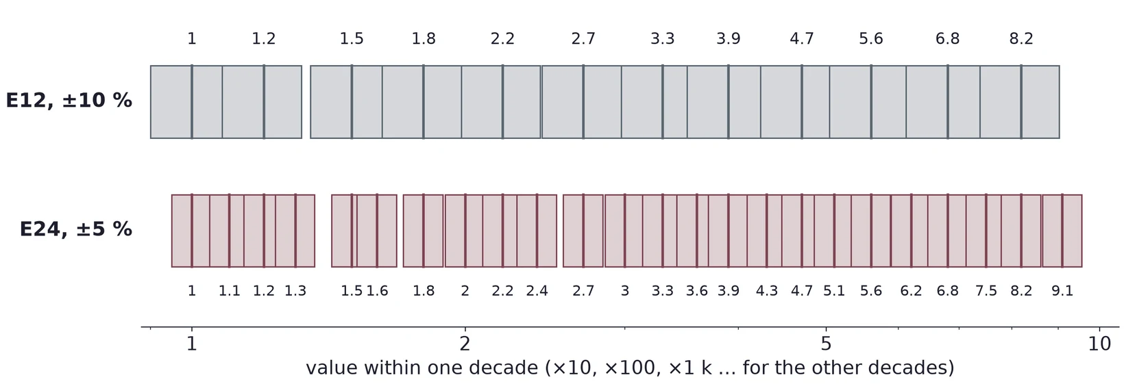
Each value's tolerance band reaches its neighbors, so any resistance is covered. 470 Ω, 22 kΩ and 2.2 MΩ are all standard values.
The datasheet gives tolerance, power and voltage
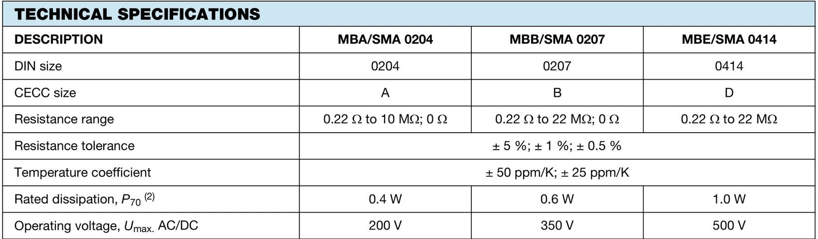
Vishay MBA/SMA 0204 metal film (document 28766): ±1 % parts, 0.4 W at 70 °C, 200 V at most. Check the series your kit uses.
Is the part in tolerance?
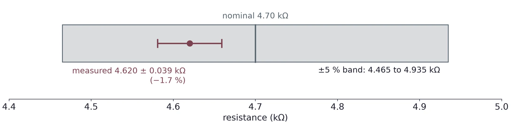
A 4.7 kΩ, ±5 % resistor that reads 4.62 kΩ is in tolerance. The error bar is the meter's uncertainty (next slide).
Your meter has an uncertainty too
Suppose the manual gives ±(0.8 % + 2 counts) on the 6.000 kΩ range:
Use your own meter's spec for the range you used. A deviation smaller than the meter's uncertainty tells you nothing.
Part 2 · An ideal source keeps its voltage
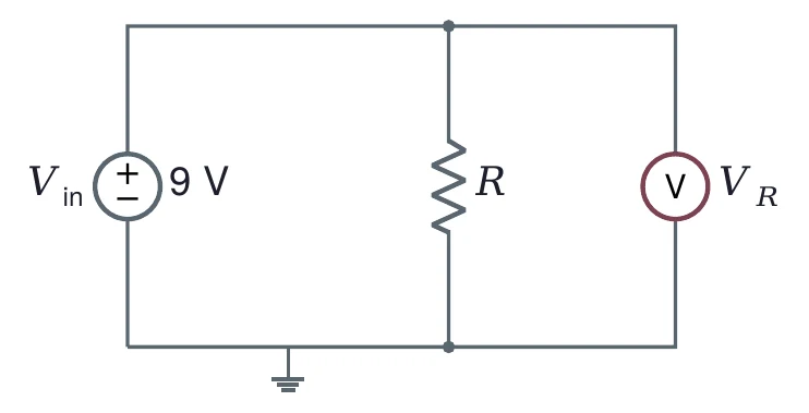
Ideal: V for any .
kΩ: 9 V, 9 mA
MΩ: 9 V, 9 µA
Ω: 9 V and 9 A?
No battery gives 9 A. A real source has a resistance inside it.
A real source has a resistance inside
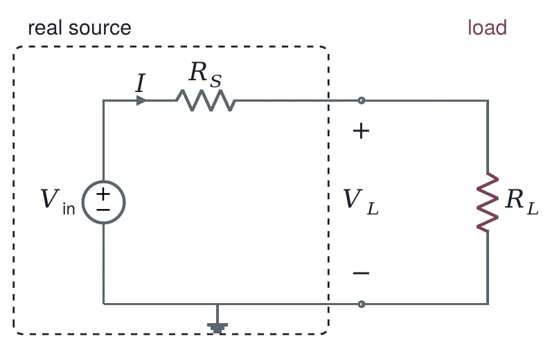
One loop, one current: .
is the source resistance, the load. Part of is lost across .
Firm and stiff sources
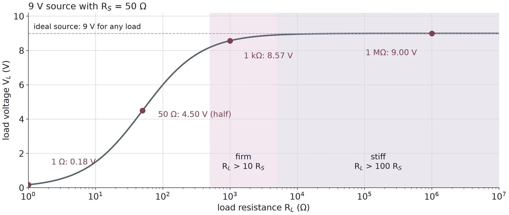
Firm: , the load gets at least 91 %. Stiff: , at least 99 %. The same source suits a large load and fails a small one.
The function generator is a 50 Ω source
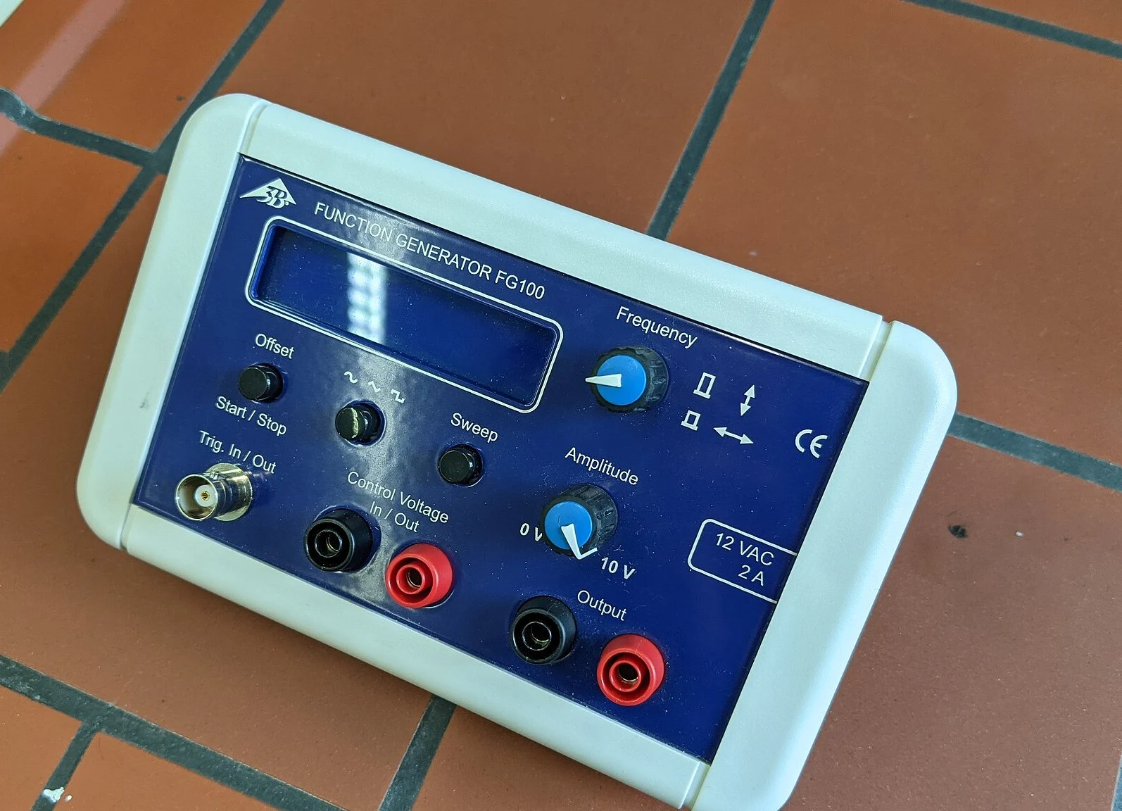
Inside: an ideal source behind 50 Ω.
The scope input is about 1 MΩ: 20 000 times larger.
So the generator is stiff for the scope, which sees the full open-circuit voltage.
Photo: Anselm Schüler, CC BY-SA 4.0.

Part 3 · The voltage divider
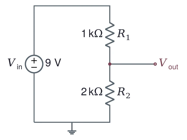
One current through both, so the voltage splits in the ratio of the resistances.
Choose the total resistance first
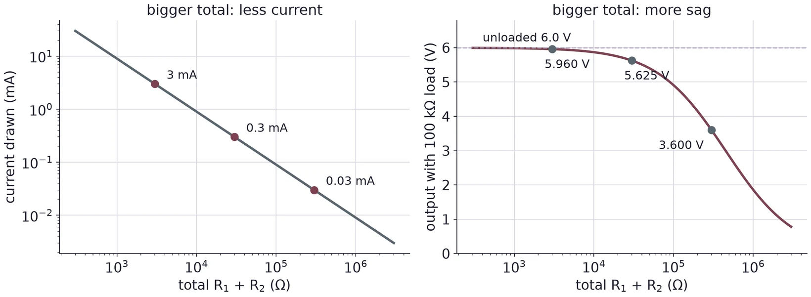
1 kΩ + 2 kΩ from 9 V: = 3 mA, 27 mW in all (9 mW in , 18 mW in ). Pick a total that suits both plots, then split it.
Several taps from one chain
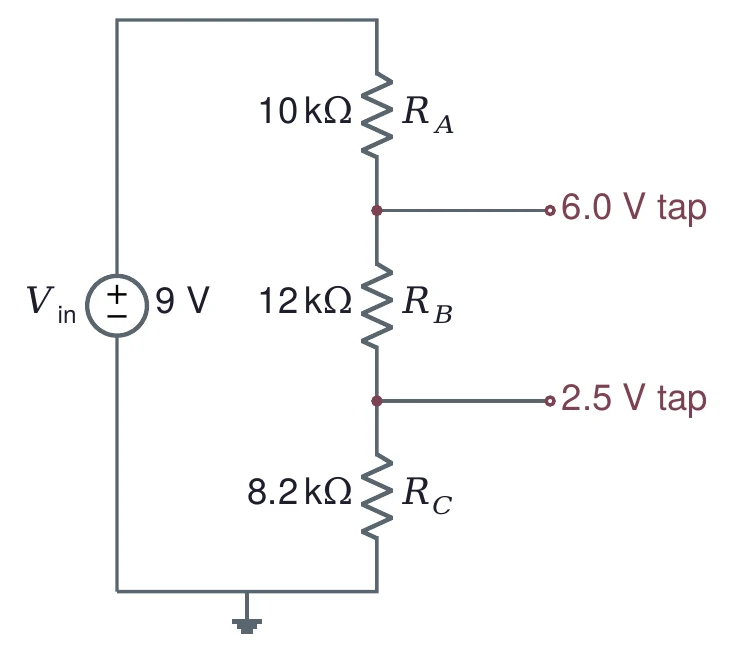
Aim: 6.0 V and 2.5 V from 9 V, about 30 kΩ total.
Each resistor gets its share of 9 V:
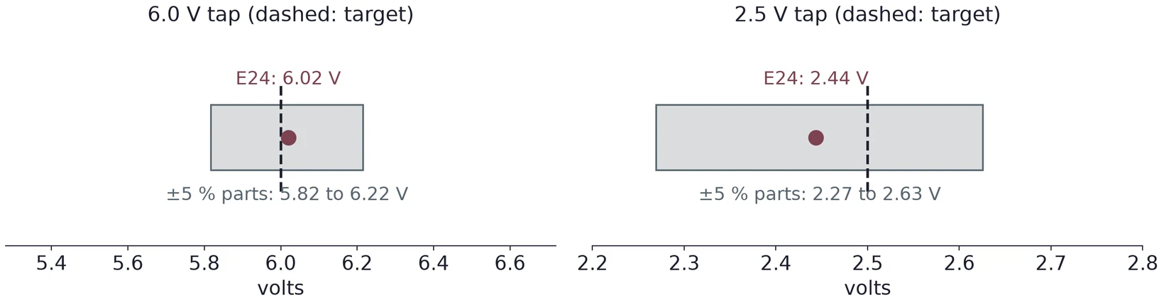
Round to standard values, then recompute
| R | Ideal | E24 |
|---|---|---|
| RA | 10.0 kΩ | 10 kΩ |
| RB | 11.67 kΩ | 12 kΩ |
| RC | 8.33 kΩ | 8.2 kΩ |
V (+0.3 %)
V (−2.3 %)
A load sits in parallel with R2
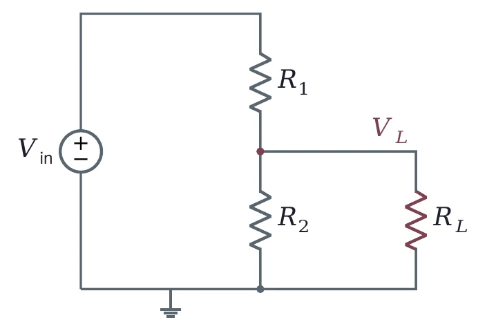
The parallel pair is always smaller than , so a load always pulls the output down.
Two 10 kΩ resistors, four loads
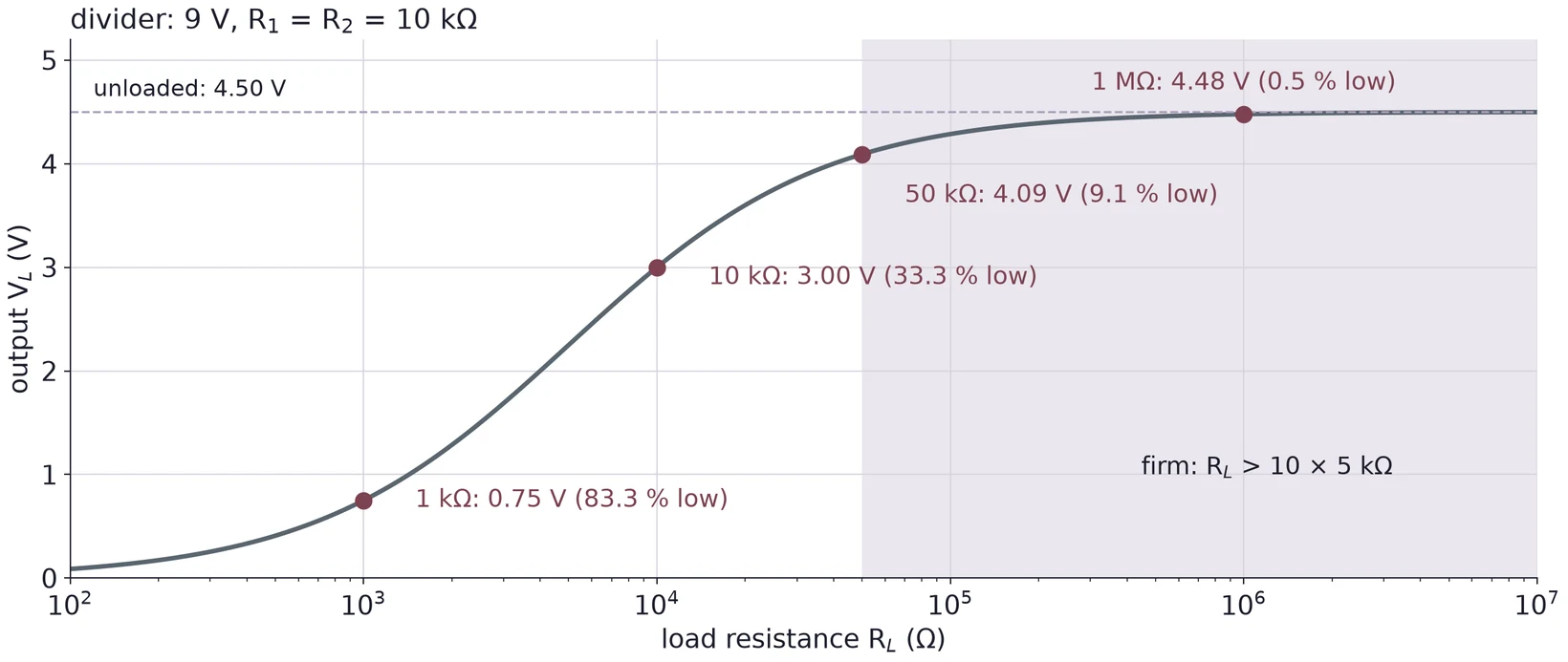
Loading effect . A 10 kΩ load costs a third of the output.
Seen from the load, a divider is a source
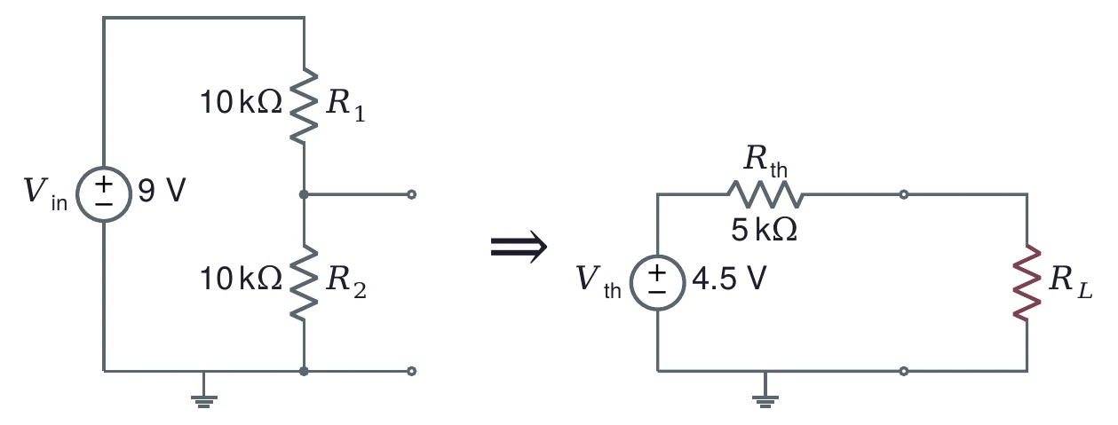
Firm when = 50 kΩ. Lab 2 shows that any circuit reduces this way: Thévenin's theorem.
Even the DMM loads the circuit
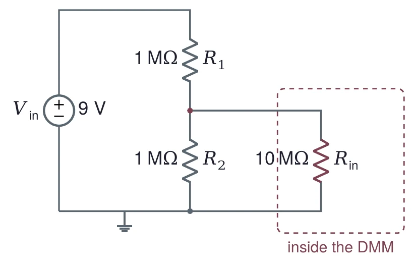
Expected: 4.50 V
Meter reads:
4.8 % low
Many DMMs have about 10 MΩ input resistance on DC volts: check yours. It matters only for megohm circuits.
Part 4 · The oscilloscope: three groups of controls
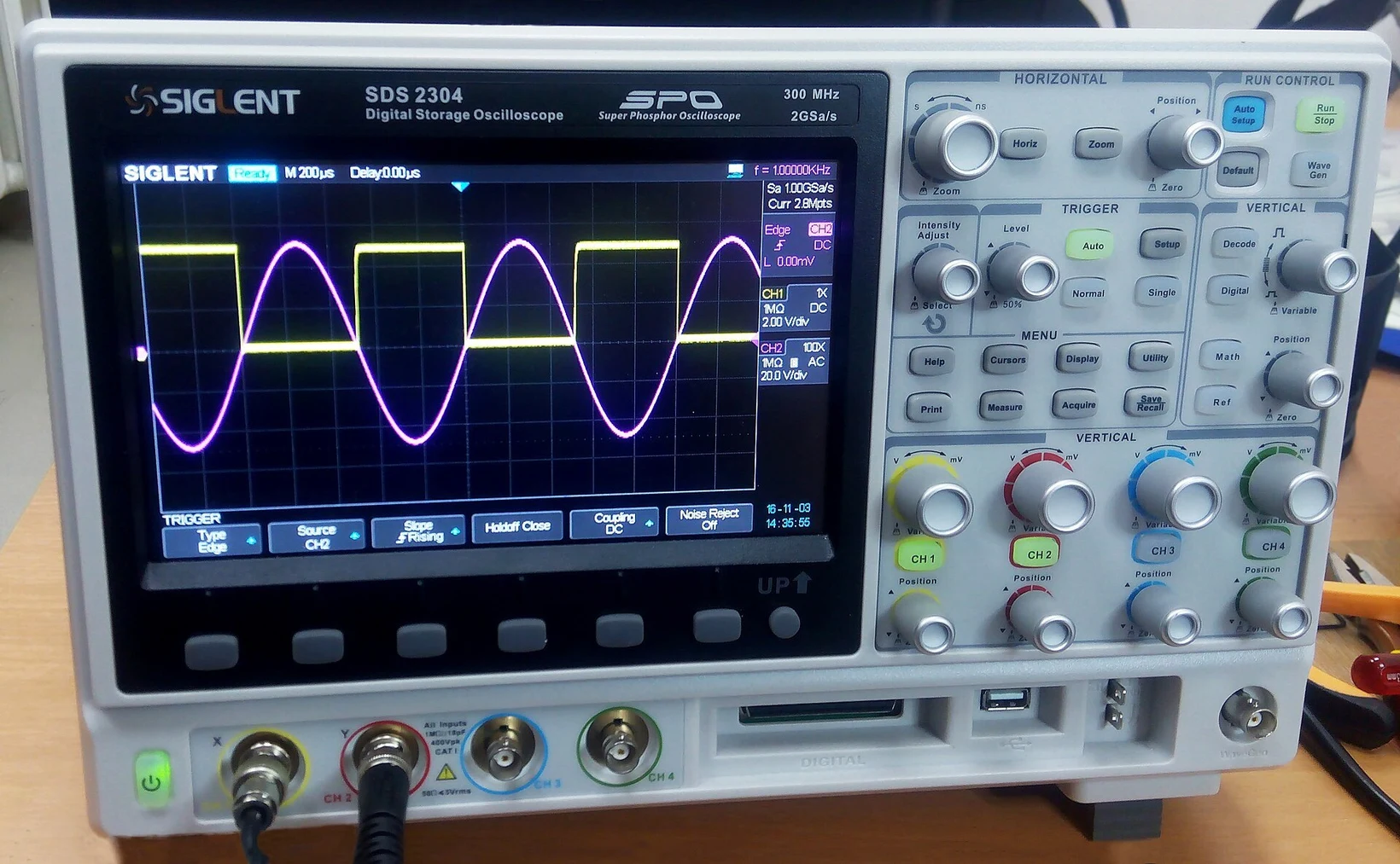
Vertical: volts per division, one per channel
Horizontal: time per division
Trigger: when each sweep starts
Photo: Wild Pancake, CC BY 4.0.

Triggering makes the trace stand still
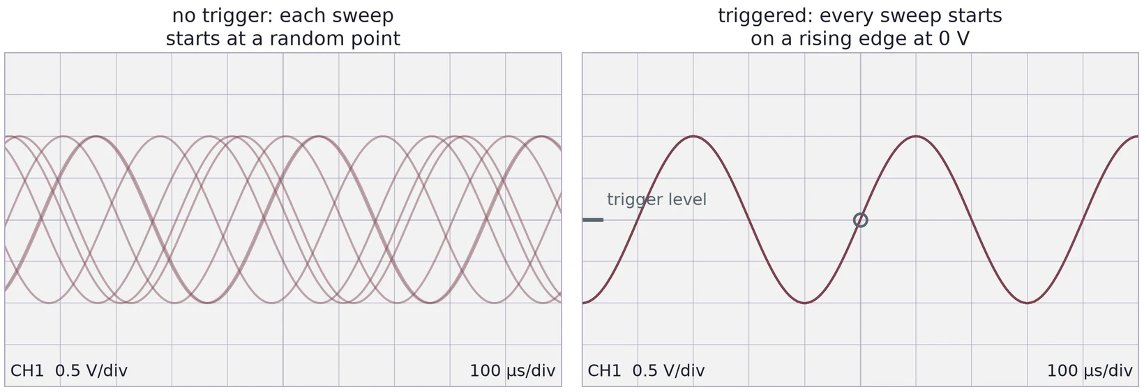
Pick the channel you are measuring as the trigger source, a rising edge, and a level inside the signal.
Reading the screen
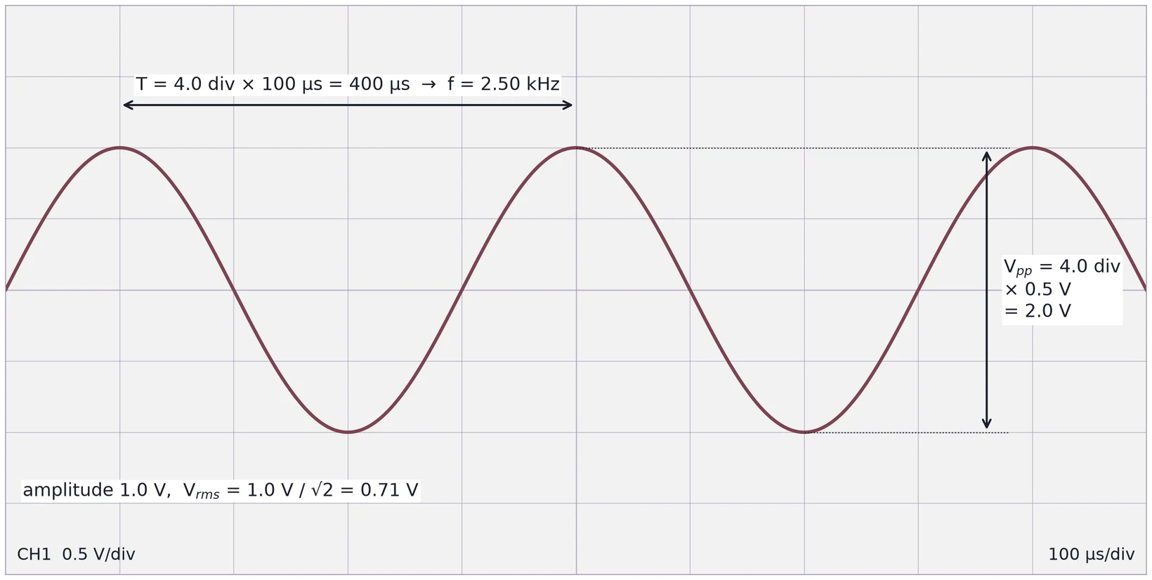
Count divisions, then multiply by the scale. .
Period and frequency carry the same relative error
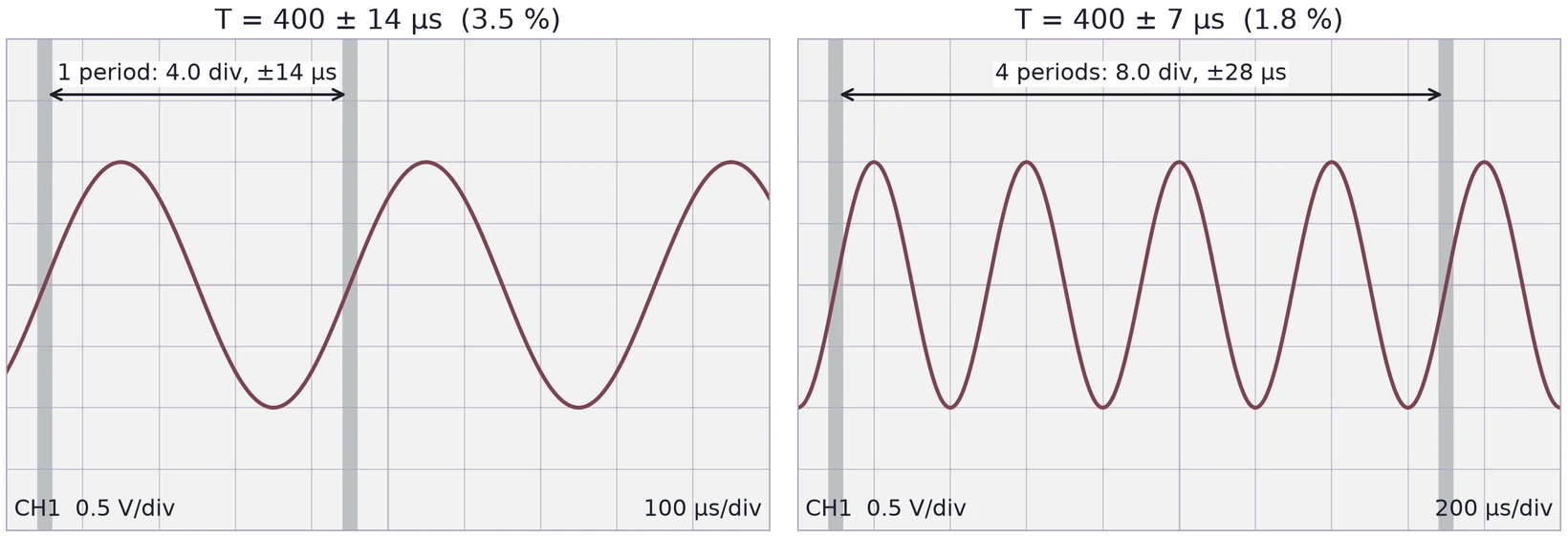
Each crossing is read to ±0.1 div. Four periods at 200 µs/div give ±7 µs per period. Report in µs and in Hz.
Check two settings before you trust a number
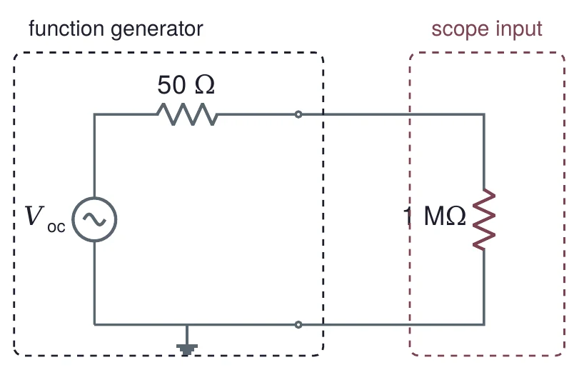
Generator load setting. Set to 1.00 Vpp in 50 Ω mode, it makes 2.00 Vpp open circuit, and the scope shows 2.00 Vpp.
Probe factor. A 10× probe on a channel set to 1× reads ten times too small.
Export the data, then plot it
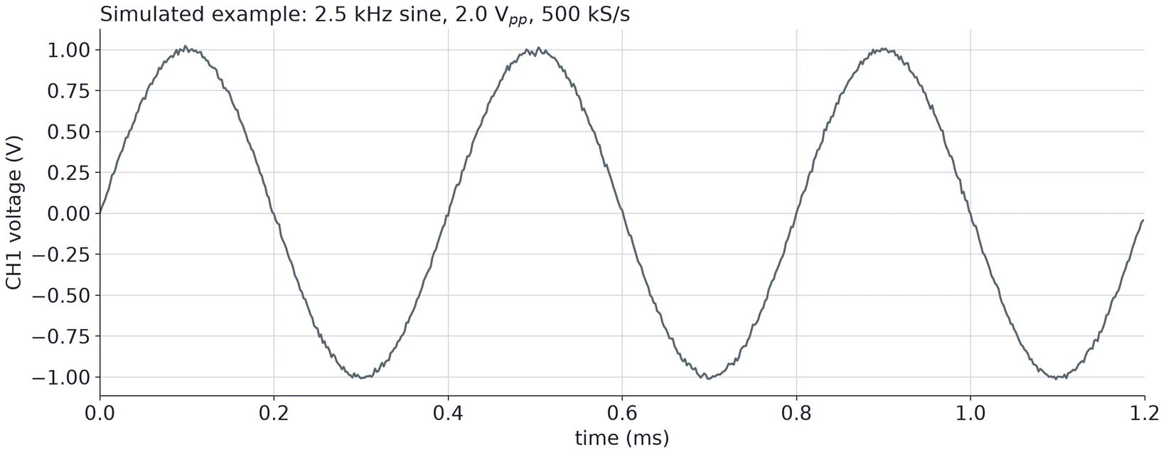
Save the trace as CSV on a USB drive. A good plot has labeled axes with units, sensible scales and a title.
Use ← → to move, Home / End to jump, and F for fullscreen.
Figure descriptions
Slide 2 · Part 1 · Lab 1 in five tasks
Lab 1 in three rows. Know the bench: Task 1, the station (breadboard, supplies, grounding), then Task 2, measuring three resistors with the DMM. Build a source: Task 3, a divider from 12 V giving 5 V, 3.3 V and 1.8 V, then Task 4, loading the divider and watching it sag. Read a signal: Task 5, triggering, measuring, exporting and plotting on the scope.
Slide 3 · The breadboard joins holes in strips of five
Breadboard connections. Columns of five holes, rows a to e and f to j, each form one node; an IC straddles the center channel so each pin has its own strip. Power rails run along the top and bottom edges; on some boards the top rails are split in the middle and need a wire to bridge the gap.
Slide 4 · Inside: one spring clip per strip
A breadboard with its backing removed, showing rows of metal spring clips, one under each strip of five holes, and the long clips of the power rails.
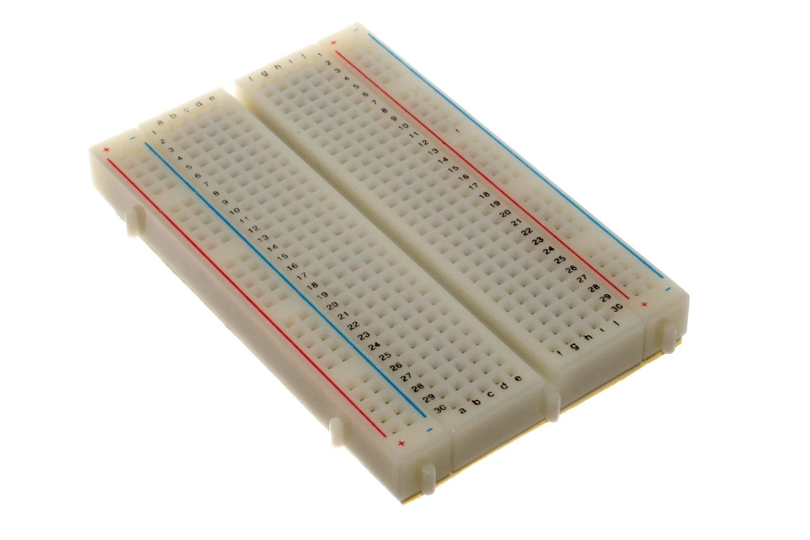
A small 400-point solderless breadboard with red and blue power rail lines along both long edges.
Slide 5 · Two kinds of power supply
A bench DC power supply with red digital displays for current (0.00 A) and voltage (11.9 V), current and voltage knobs, and red and black output terminals.
Slide 7 · The DMM: across for volts, in series for amps
A handheld digital multimeter with a large display, a rotary range switch and four input jacks at the bottom.
Two circuits. Left: a voltmeter connected across a resistor R powered by a source V_S, labeled voltage: across the part. Right: an ammeter in series between the source V_S and the resistor R, labeled current: in series.
Slide 8 · Read the color code
A through-hole resistor with brown, black, orange and gold bands: 10 kilohms, plus or minus 5 percent.
Slide 9 · Standard values come in E-series
The E12 and E24 standard values in one decade on a log scale, each drawn with its tolerance band. E12 values 1, 1.2, 1.5, 1.8, 2.2, 2.7, 3.3, 3.9, 4.7, 5.6, 6.8, 8.2 with plus or minus 10 percent bands; E24 values from 1 to 9.1 with plus or minus 5 percent bands. Neighboring bands touch or overlap, so the decade is covered.
Slide 10 · The datasheet gives tolerance, power and voltage
Technical specifications table from the Vishay MBA/SMA 0204, MBB/SMA 0207 and MBE/SMA 0414 datasheet: resistance range 0.22 ohm to 10 or 22 megohm; tolerance plus or minus 5, 1 or 0.5 percent; temperature coefficient 50 or 25 ppm per kelvin; rated dissipation at 70 degrees C of 0.4, 0.6 and 1.0 W; operating voltage 200, 350 and 500 V.
Slide 11 · Is the part in tolerance?
A resistance axis from 4.4 to 5.0 kilohms. A shaded band from 4.465 to 4.935 kilohms is the plus or minus 5 percent tolerance of a 4.70 kilohm resistor, marked at its nominal value. A measured point at 4.620 kilohms with an error bar of plus or minus 0.039 kilohms (minus 1.7 percent) lies inside the band.
Slide 12 · Your meter has an uncertainty too
A handheld digital multimeter with a large display, a rotary range switch and four input jacks at the bottom.
Slide 13 · Part 2 · An ideal source keeps its voltage
A 9 V source V_in connected across a resistor R, with a voltmeter V_R across R. The bottom wire is grounded.
Slide 14 · A real source has a resistance inside
A real source: inside a dashed box, the source V_in in series with a source resistance R_S, carrying current I to two output terminals. The output voltage V_L appears across the terminals, which connect to a load resistor R_L outside the box.
Slide 15 · Firm and stiff sources
Load voltage against load resistance, from 1 ohm to 10 megohms on a log axis, for a 9 V source with R_S of 50 ohms. The curve rises from 0.18 V at 1 ohm through 4.50 V at 50 ohms (half) to 8.57 V at 1 kilohm and 9.00 V at 1 megohm, approaching the dashed 9 V line of an ideal source. Shaded regions mark firm (R_L above 10 R_S) and stiff (R_L above 100 R_S).
Slide 16 · The function generator is a 50 Ω source
A small laboratory function generator with a frequency display, waveform and amplitude controls, and output jacks.
Slide 17 · Part 3 · The voltage divider
A voltage divider: a 9 V source V_in drives R_1 of 1 kilohm in series with R_2 of 2 kilohms to ground; V_out is taken at the node between them.
Slide 18 · Choose the total resistance first
Two plots against the total resistance of a 6 V divider from 9 V, from 300 ohms to 3 megohms. Left, log scales: the current drawn falls from 3 mA at 3 kilohms to 0.3 mA at 30 kilohms and 0.03 mA at 300 kilohms. Right: the output with a 100 kilohm load stays near the unloaded 6.0 V for small totals (5.960 V at 3 kilohms, 5.625 V at 30 kilohms) and drops to 3.600 V at 300 kilohms.
Slide 19 · Several taps from one chain
A three-resistor chain from a 9 V source: R_A 10 kilohms, R_B 12 kilohms and R_C 8.2 kilohms to ground, with a 6.0 V tap between R_A and R_B and a 2.5 V tap between R_B and R_C.
Slide 20 · Round to standard values, then recompute
Two panels for the 6.0 V and 2.5 V taps. Each shows the target as a dashed line, the output with exact E24 parts as a dot (6.02 V and 2.44 V), and a band for the worst case with plus or minus 5 percent parts: 5.82 to 6.22 V and 2.27 to 2.63 V.
Slide 21 · A load sits in parallel with R2
A loaded voltage divider: source V_in drives R_1 in series with R_2 to ground; a load resistor R_L connects from the middle node to ground, in parallel with R_2, and the load voltage V_L is taken at that node.
Slide 22 · Two 10 kΩ resistors, four loads
Output voltage against load resistance, from 100 ohms to 10 megohms on a log axis, for a divider of two 10 kilohm resistors from 9 V. The unloaded output is 4.50 V. Marked points: 1 kilohm gives 0.75 V (83.3 percent low), 10 kilohms 3.00 V (33.3 percent low), 50 kilohms 4.09 V (9.1 percent low) and 1 megohm 4.48 V (0.5 percent low). Loads above 50 kilohms, ten times the 5 kilohm source resistance, are shaded as firm.
Slide 23 · Seen from the load, a divider is a source
Left: a 9 V source with two 10 kilohm resistors in series, the output taken between them. An arrow points to the right: the equivalent source V_th of 4.5 V in series with R_th of 5 kilohms, driving a load R_L.
Slide 24 · Even the DMM loads the circuit
A divider of two 1 megohm resistors from 9 V, with the DMM's 10 megohm input resistance R_in connected across the lower resistor, shown in a dashed box labeled inside the DMM.
Slide 25 · Part 4 · The oscilloscope: three groups of controls
A four-channel digital storage oscilloscope showing a sine wave and a square wave, with vertical, horizontal and trigger controls to the right of the screen.
Slide 26 · Triggering makes the trace stand still
Two scope screens at 0.5 V per division and 100 microseconds per division. Left, no trigger: seven sweeps of a sine wave start at random points and overlap into a blur. Right, triggered: every sweep starts on a rising edge through 0 V at the center of the screen, so the traces sit on top of each other as one stable sine wave.
Slide 27 · Reading the screen
A scope screen at 0.5 V per division and 100 microseconds per division showing a sine wave. One period spans 4.0 divisions, 400 microseconds, so f = 2.50 kHz. Peak to peak spans 4.0 divisions, 2.0 V. Amplitude 1.0 V, RMS 0.71 V.
Slide 28 · Period and frequency carry the same relative error
Two scope screens of a 2.5 kHz sine at 0.5 V per division. Left, 100 microseconds per division: one period spans 4.0 divisions, read to plus or minus 14 microseconds, so T is 400 plus or minus 14 microseconds (3.5 percent). Right, 200 microseconds per division: four periods span 8.0 divisions, read to plus or minus 28 microseconds, so T is 400 plus or minus 7 microseconds per period (1.8 percent). Shaded strips mark plus or minus 0.1 division at each crossing.
Slide 29 · Check two settings before you trust a number
A function generator modeled as an AC source V_oc in series with 50 ohms, inside a dashed box, connected to the scope input, a 1 megohm resistor in a second dashed box.
Slide 30 · Export the data, then plot it
A plot of simulated exported scope data: CH1 voltage in volts against time in milliseconds from 0 to 1.2 ms, a 2.5 kHz sine of 2.0 V peak to peak with slight noise, with labeled axes, a grid and a title.