1 Where Lab 1 Sits
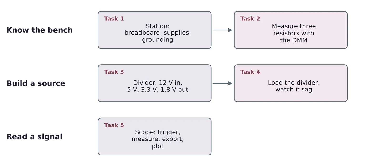
Lab 1 has three parts. First you learn the bench and measure parts with the digital multimeter (DMM). Then you build a source out of resistors and watch what happens when something draws current from it. Last, you read a signal on the oscilloscope and save it.
1.1 Task map
| Lab 1 task | What you do | Concept & section |
|---|---|---|
| 1 | Learn the station: breadboard, supplies, grounding | The bench (§2) |
| 2 | Measure 470 Ω, 22 kΩ and 2.2 MΩ resistors; compare with tolerance | The DMM and resistors (§3) |
| 3 | Design a divider that gives 5, 3.3 and 1.8 V from 12 V | Sources (§4), the voltage divider (§5) |
| 4 | Load a divider of two 22 kΩ resistors; find the loading effect | Loading (§6) |
| 5 | Trigger, measure, export and plot a 1 kHz sine | The oscilloscope (§7) |
Every task needs an error analysis. Section 8 collects the main error sources for each kind of measurement.
2 The Bench
2.1 The breadboard
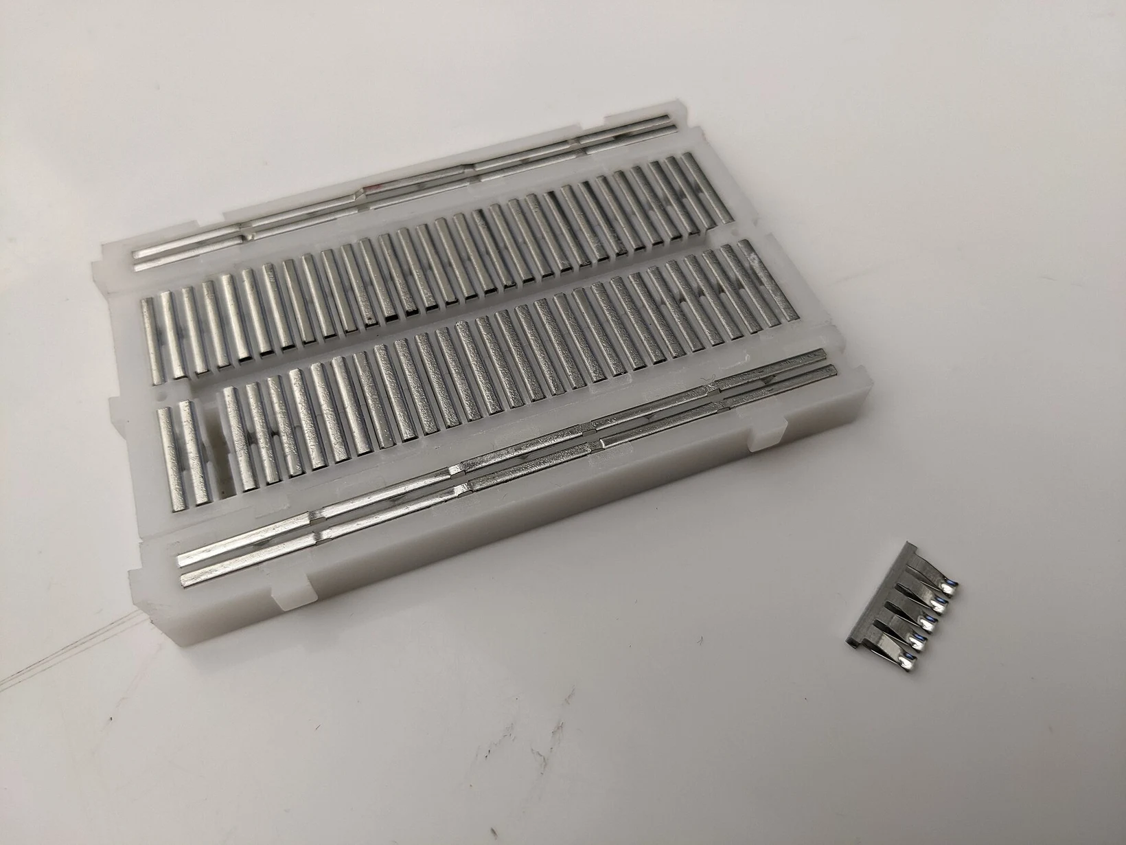
A solderless breadboard holds parts without solder. Under each strip of five holes sits one metal spring clip, so the five holes are one electrical node. A lead pushed into any of them is connected to the other four. The two halves of the board, rows a to e and f to j, are separated by a center channel. A chip in a dual in-line package (DIP) sits across that channel, so each of its pins lands in its own strip.
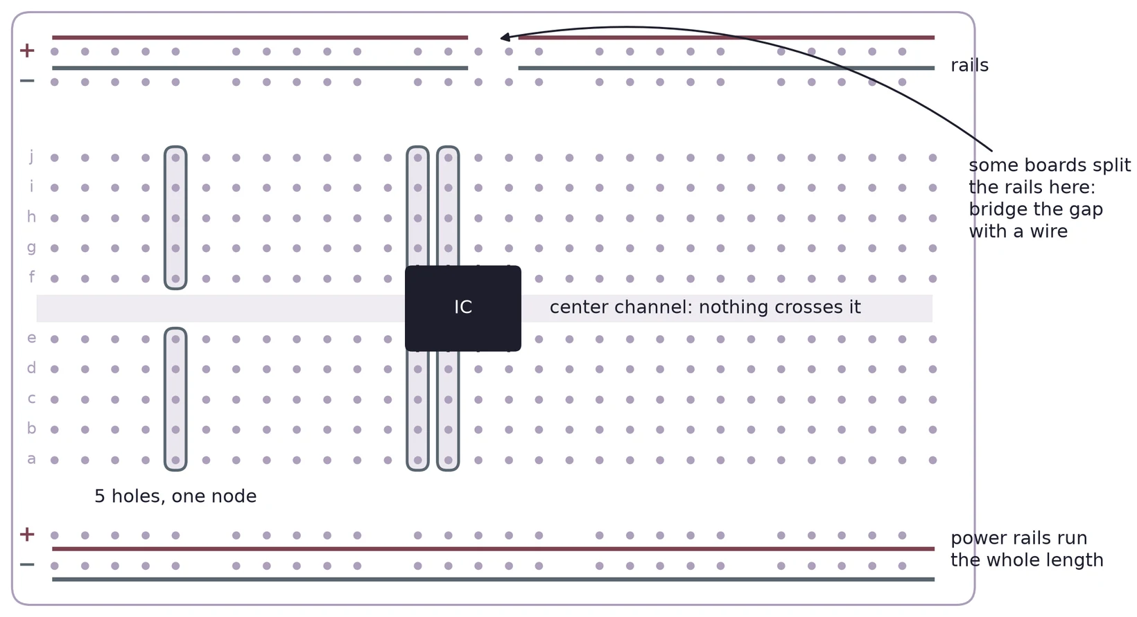
The long rows along the edges are the power rails, usually marked with a red (+) and a blue (−) line. Use one rail for the supply and one for ground, and keep that choice the same on every board you build. On some long boards, each rail is split into two halves. If half of your circuit seems dead, check for a split rail and bridge it with a short wire.

2.2 Two kinds of power supply
Your station can power a circuit in two ways. An integrated supply is built into the prototyping station. It may have fixed outputs, adjustable ones, or both, and its ground is shared with the rest of the station. An external bench supply is a separate box with its own voltage and current knobs. Its outputs are often floating: the − terminal is not connected to anything until you connect it to your circuit's ground.
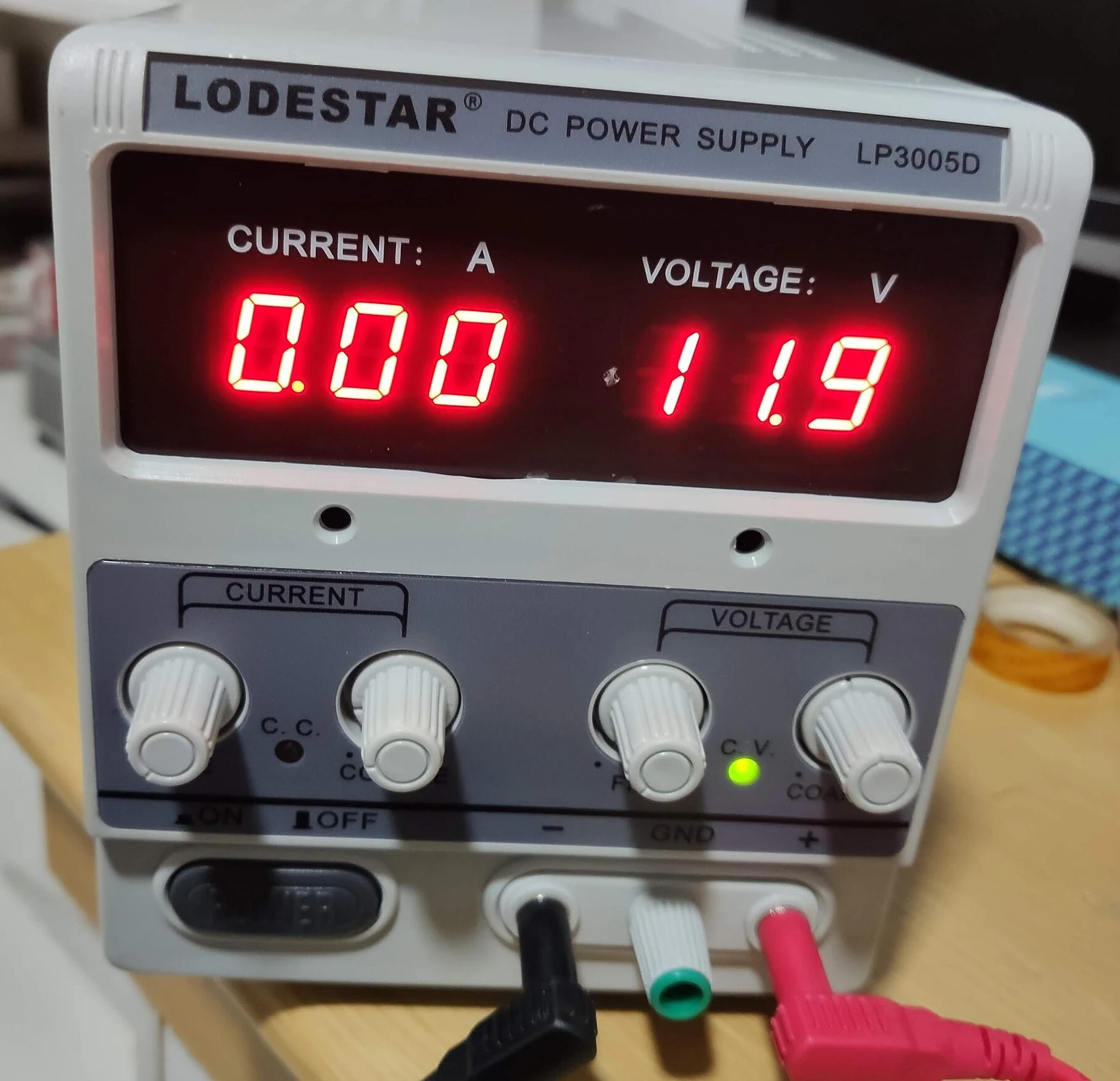

A bench supply holds its output voltage until the load asks for more than the current limit. Then it switches to holding the current at the limit, and the voltage drops. Set the limit a little above what your circuit should draw. A wiring mistake then shows up as a sagging voltage instead of a hot part.
2.3 One ground for every instrument
A voltage is always measured between two points. "The output is 5 V" means 5 V above ground, so every instrument and every supply must agree on where ground is. Most strange readings in a first lab come from a missing or wrong ground connection.
| Mistake | What you see | Fix |
|---|---|---|
| Supply − not tied to circuit ground | Readings drift or make no sense | Wire the supply's − terminal to the ground rail |
| Two supplies, no common ground | One part of the circuit floats | Join their − terminals |
| Scope ground clip on a signal node | That node shorts to earth | Clip the ground lead to circuit ground only |
| Split rail left open | Half the board is dead | Bridge the gap with a wire |
On most bench oscilloscopes and function generators, the outer shell of each BNC connector is tied to mains earth. Every scope ground clip is therefore the same node, and so is the generator's ground. Clip a ground lead to a node that is not ground and you short that node to earth through the instruments.
(a) You power a circuit from an external bench supply and measure its output with the scope. The trace jumps around and the DMM shows a different value every time you touch the board. What is the first connection you check?
(b) A circuit needs +5 V and +12 V from two separate supplies. Draw how the four supply terminals connect to the board.
3 The DMM and Resistors
3.1 Connecting the meter
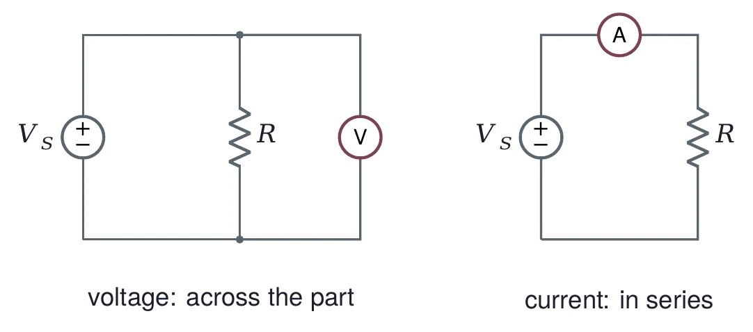
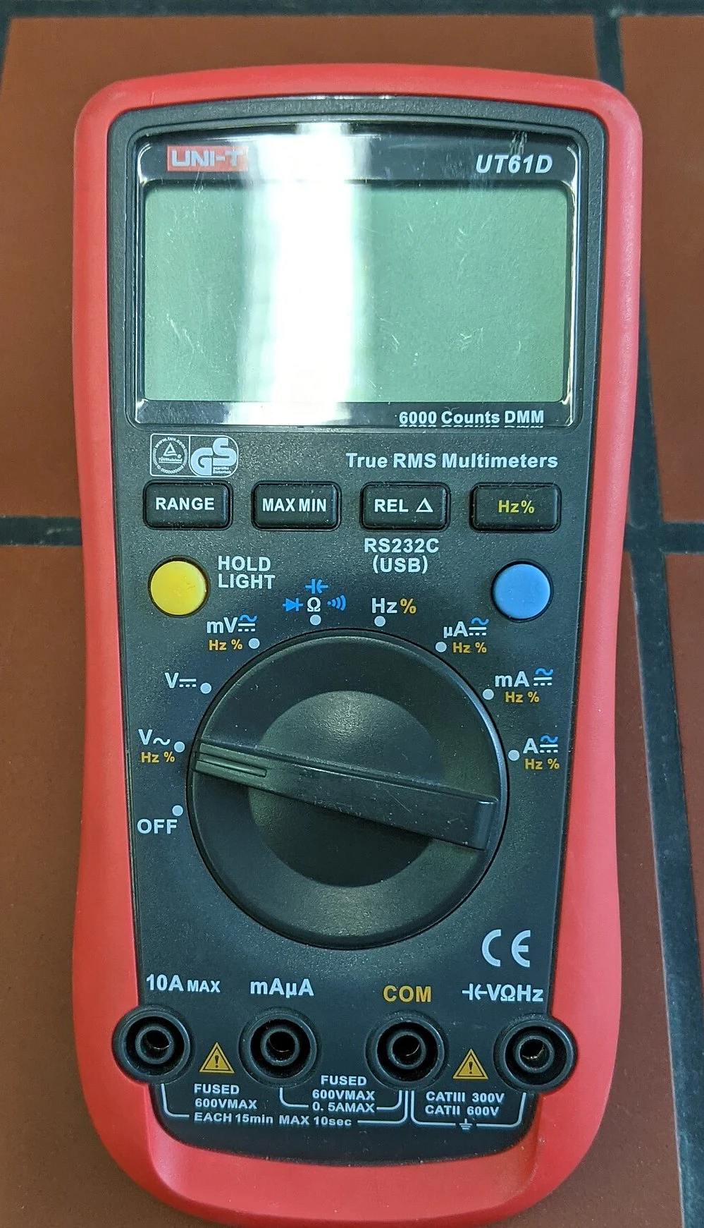
A DMM measures voltage, current and resistance. To measure a voltage, connect the meter across the part, in parallel with it. To measure a current, break the circuit and put the meter in series, so the current flows through it. The current jacks are separate (A or mA), and the meter's resistance there is small. Leave the red lead in the current jack and switch to volts, and you short whatever you touch.
To measure resistance, take the part out of the circuit and turn the power off. In circuit, the meter also sees every other path between the two leads, and a powered circuit can damage the meter's resistance range.

3.2 The color code
Through-hole resistors carry their value in colored bands. On a four-band resistor, the first two bands are digits, the third is the power of ten, and the fourth is the tolerance.
| Color | Digit | Color | Digit | Tolerance band |
|---|---|---|---|---|
| black | 0 | green | 5 | brown ±1 % |
| brown | 1 | blue | 6 | red ±2 % |
| red | 2 | violet | 7 | gold ±5 % |
| orange | 3 | gray | 8 | silver ±10 % |
| yellow | 4 | white | 9 |
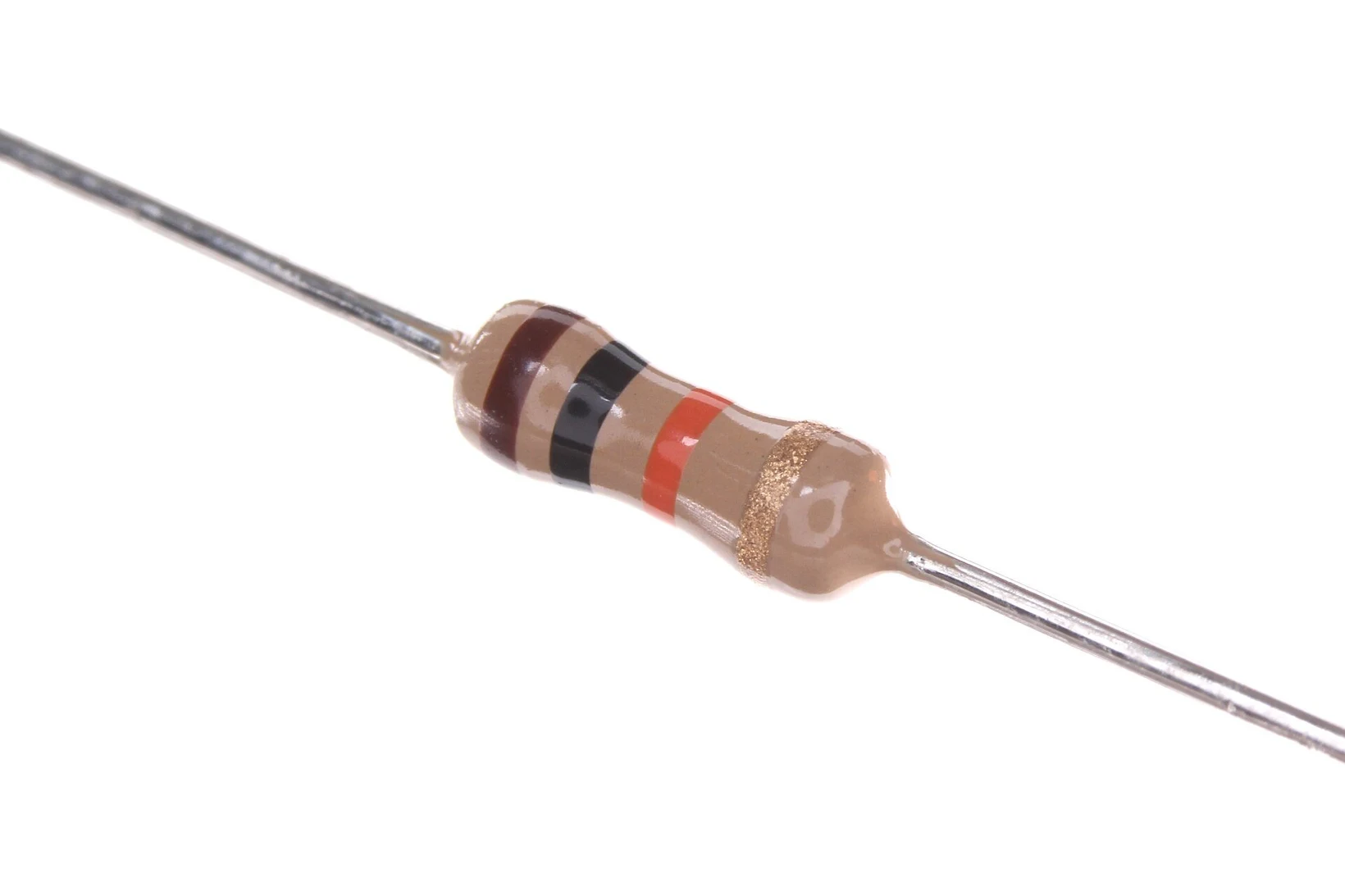

Precision resistors often have five bands: three digits, the multiplier, then the tolerance. When you are unsure which end to start from, measure it.
3.3 Standard values
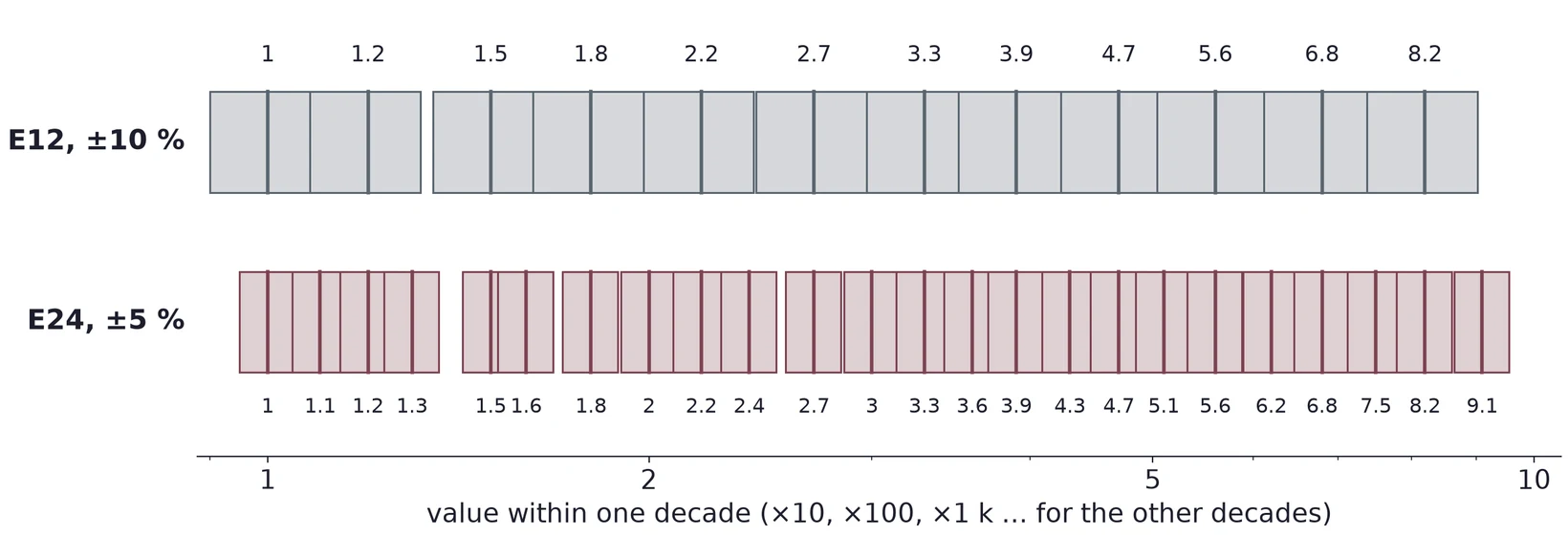
Resistors are not made in every value. They come in E-series: the E12 series has 12 values per decade for ±10 % parts, and the E24 series has 24 values per decade for ±5 % parts. The values are spaced so that each one's tolerance band reaches its neighbors. Any resistance you might need is then within tolerance of some standard part. The same values repeat in every decade: 2.2 Ω, 22 Ω, 220 Ω, 2.2 kΩ and so on.
3.4 What the datasheet says
A resistor's datasheet gives more than its value. Figure 9 is the specification table of a common family of metal film resistors. Three lines matter in this lab. The tolerance tells you how far a new part may be from its nominal value. The rated dissipation tells you how much power it can turn into heat: 0.4 W for the smallest size, at 70 °C. The operating voltage is the most you may put across it.
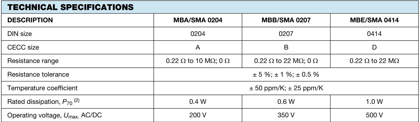
Your kit may hold carbon film parts from another maker. Read the band colors for the tolerance, and look up the series for the power rating.
3.5 Deviation from nominal
The percentage deviation compares what you measured with what the bands say:
The DMM reads 4.62 kΩ. The deviation is (4.62 − 4.70)/4.70 × 100 % = −1.7 %. A ±5 % part may lie anywhere from 0.95 × 4.70 = 4.465 kΩ to 1.05 × 4.70 = 4.935 kΩ, so this one is in tolerance.
3.6 The meter's own uncertainty
The DMM is not perfect either. Its manual gives the accuracy for each range, usually as a percentage of the reading plus a number of counts (steps of the last digit). A deviation smaller than the meter's uncertainty cannot be told apart from zero.
Suppose the manual gives ±(0.8 % + 2 counts) on the 6.000 kΩ range, where one count is 0.001 kΩ. For a reading of 4.620 kΩ:
So kΩ, or ±0.84 %. The −1.7 % deviation above is about twice that, so it is a real difference.
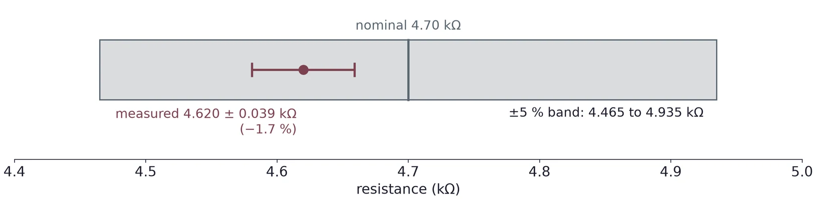
These numbers are an example. Find the specification for your own meter and the range you used. At the extremes, other errors join in: the resistance of the test leads matters for a few ohms, and your fingers on both leads put your body's resistance in parallel with a megohm resistor.
(a) A resistor has bands red, red, yellow, gold. What is its nominal value, and what range of values is in tolerance?
(b) A 1.5 kΩ, ±1 % resistor reads 1.48 kΩ. Is it in tolerance? With the meter specification of §3.6 on the same range, can you be sure?
(c) Why might a 2.2 MΩ resistor read low if you hold both leads between your fingers?
4 Sources
4.1 The ideal source
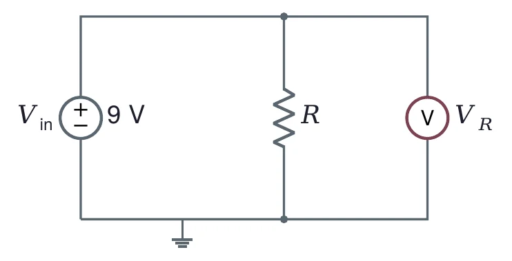
An ideal voltage source keeps its voltage whatever you connect to it. Connect a resistor across an ideal 9 V source and the voltage across it, , is 9 V for every . With 1 kΩ the current is 9 mA, and with 1 MΩ it is 9 µA. With 1 Ω, the ideal source would push 9 A. No 9 V battery can do that.
4.2 A real source has a resistance inside
A real source behaves like an ideal one in series with a small resistance , the source resistance. The load is in series with , so the same current flows through both (). Ohm's law around the loop gives the load voltage:
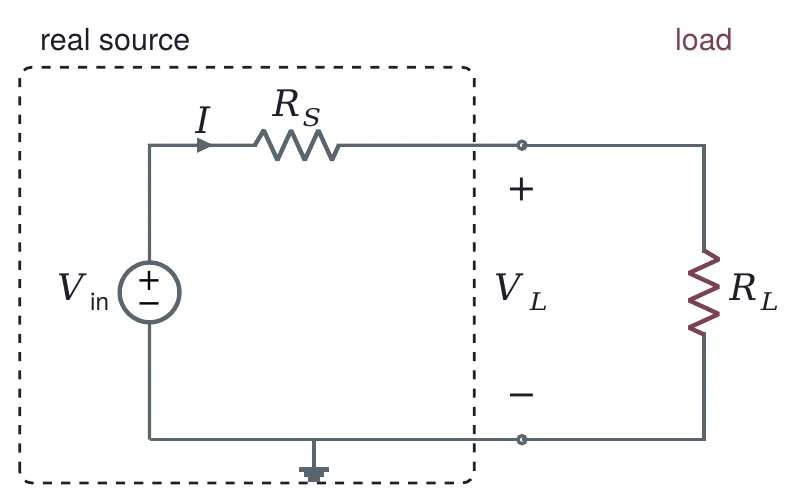
The voltage across is lost inside the source. How much is lost depends on the load.
With = 1 kΩ: V, 95.2 % of 9 V.
With = 1 Ω: V. The current is 0.18 A, not 9 A, and nearly all of the voltage is lost across .
With = 1 MΩ: V, effectively 9 V.
4.3 Firm and stiff
Figure 13 shows for every load from 1 Ω to 10 MΩ. When the load gets exactly half. Two rules of thumb name the region where the source is close to ideal:
A source is firm if : the load gets at least = 91 % of the open-circuit voltage.
A source is stiff if : the load gets at least = 99 %.
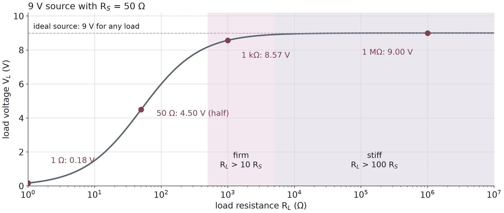
"Stiff" is not a property of the source alone. The same 50 Ω source is stiff for a 10 kΩ load and useless for a 10 Ω one.
4.4 The function generator is a 50 Ω source
The function generator on your bench is a source of this kind. Inside, an ideal AC source sits behind a 50 Ω output resistance. The scope input is about 1 MΩ, so the generator is stiff for it: the scope sees the full open-circuit voltage.
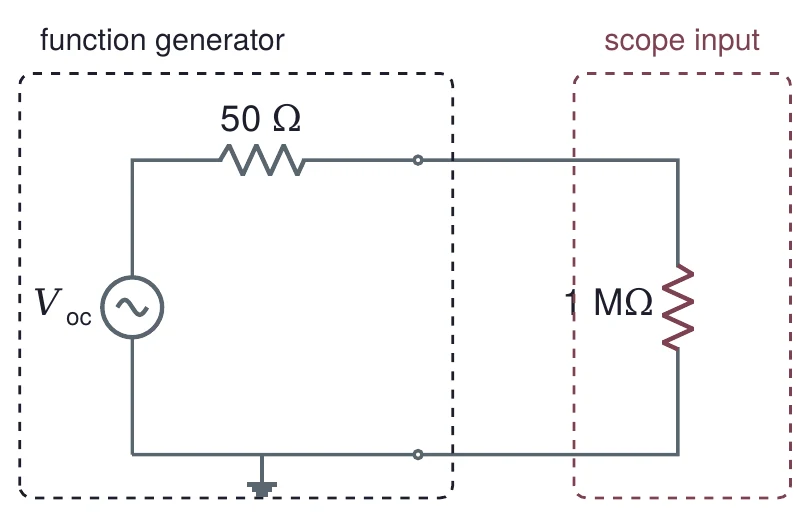
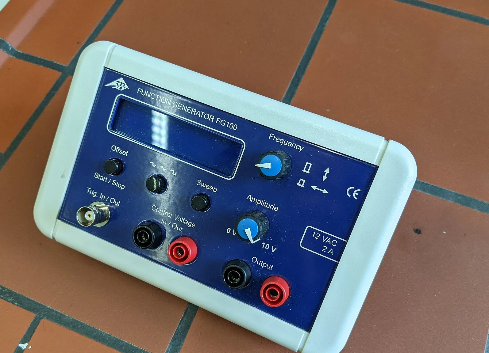

Many generators have a load setting, 50 Ω or High-Z, that changes only what the display shows. In 50 Ω mode, the display assumes a 50 Ω load, which gets half of . Set 1.00 Vpp in that mode and the generator makes 2.00 Vpp open circuit: a 50 Ω load would get 1.00 Vpp, but the scope's 1 MΩ gets 2.00 Vpp. If your scope shows twice what you set, check this setting before anything else.
(a) A 12 V source has = 2 Ω. What does a 100 Ω load get? Is the source firm, stiff, or neither, for that load?
(b) For the same source, what is the smallest load for which it is stiff?
(c) A generator in 50 Ω mode is set to 300 mVpp. What does the scope show at its 1 MΩ input? What would it show if you added a 50 Ω resistor across the scope input?
5 The Voltage Divider
5.1 Two resistors in series
Two resistors in series across a source carry the same current, so the source voltage splits between them in the ratio of their resistances. The output, taken across , is
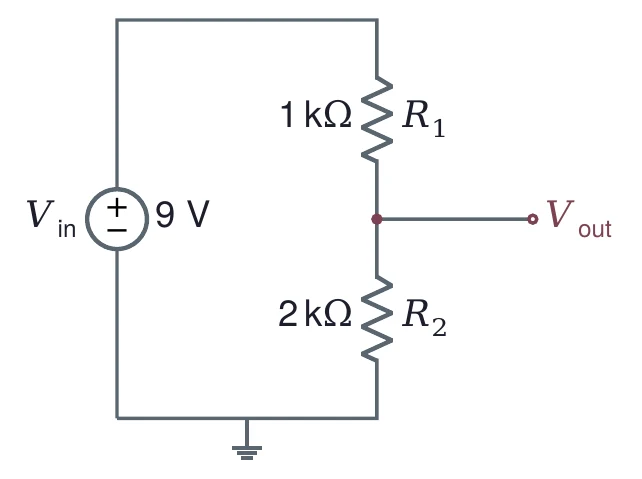
Equation (3) holds only while nothing draws current from the output. Section 6 deals with the load.
5.2 Choose the total resistance first
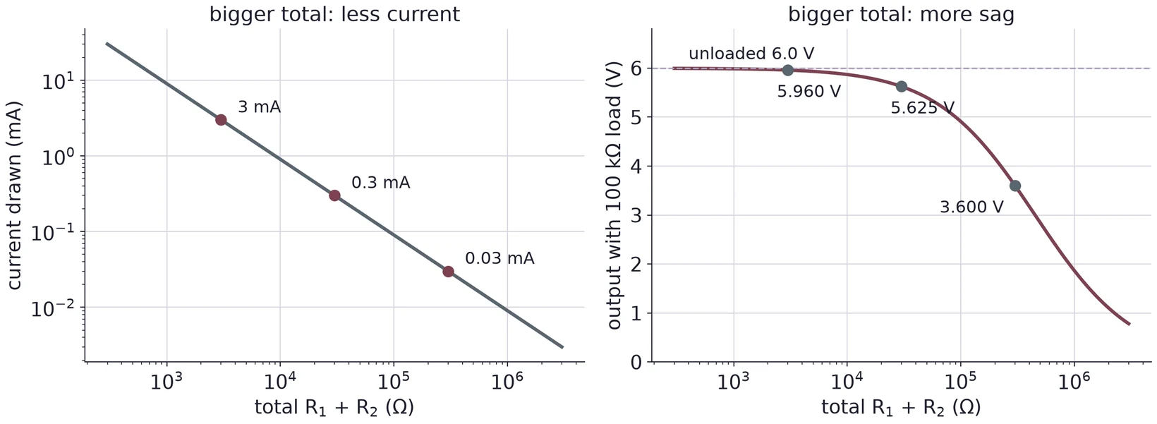
Only the ratio of and sets the output. The total sets the current, and with it the power:
mA. The chain uses = 27 mW: = 9 mW in and 18 mW in . Both are far below the 0.4 W of Figure 9.
Small resistors draw more current, heat up and drain a battery. Large resistors make a weak source that sags as soon as a load is connected (§6). A design starts by picking a total that balances the two, then splits it.
5.3 Several outputs from one chain
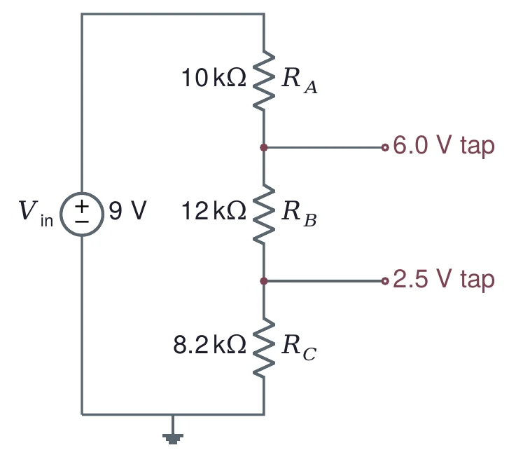
A chain of three or more resistors gives several outputs at once. Each resistor gets the share of the total voltage that drops across it. Work from the bottom up: the bottom resistor sets the lowest tap, the next one the difference to the second tap, and so on.
Aim for about 30 kΩ in total. The bottom resistor carries 2.5 V, the middle one 6.0 − 2.5 = 3.5 V, and the top one 9 − 6.0 = 3.0 V:
The nearest E24 values are 8.2 kΩ, 12 kΩ and 10 kΩ, 30.2 kΩ in total. Recompute with the real values:
The chain draws 9 V/30.2 kΩ = 0.30 mA and uses 2.7 mW.
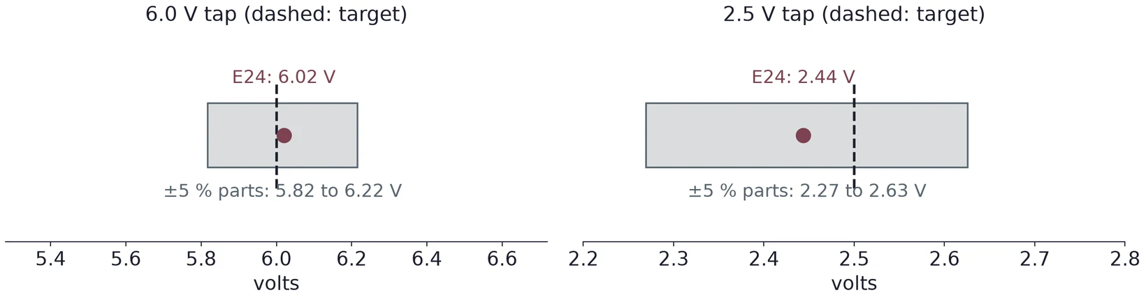
Rounding is one error. Tolerance is the other: with ±5 % parts, each resistor can be off by 5 %, and the taps move with them. The worst case for a tap puts every resistor below it 5 % high and every one above it 5 % low, or the other way round. For the 2.5 V tap that gives 2.27 to 2.63 V; for the 6.0 V tap, 5.82 to 6.22 V. If a tap must be exact, two standard values in series or a potentiometer can trim it.
(a) Design a chain that gives 10 V and 4 V from 15 V with about 47 kΩ in total. Choose E24 values, then recompute both outputs and their errors.
(b) If the bottom resistor in (a) is 5 % high and the others are exact, which way does each tap move?
(c) What limits how small the total resistance may be? What limits how large?
6 Loading
6.1 A load sits in parallel with R2
Connect a load to a divider's output and it sits in parallel with . The pair has a smaller resistance than alone,
so the output drops:
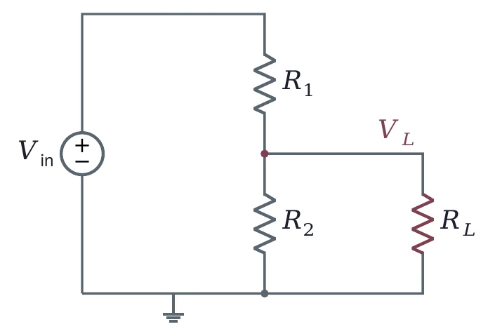
The loading effect measures how much the output fell:
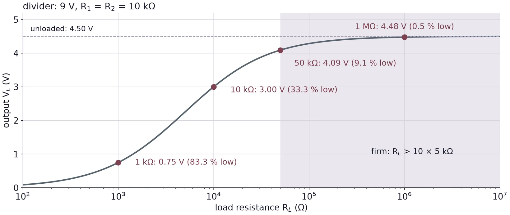
Unloaded, the output is 4.50 V. With a 10 kΩ load, = 5 kΩ and V, a loading effect of 33.3 %. With a 1 kΩ load, = 0.909 kΩ and = 0.75 V (83.3 %). With 1 MΩ, = 4.48 V (0.5 %).
6.2 Seen from the load, a divider is a source
Section 4 had a source with a resistance inside. A divider behaves the same way. Seen from its output, it is an ideal source , the unloaded output, behind a resistance , which is and in parallel:
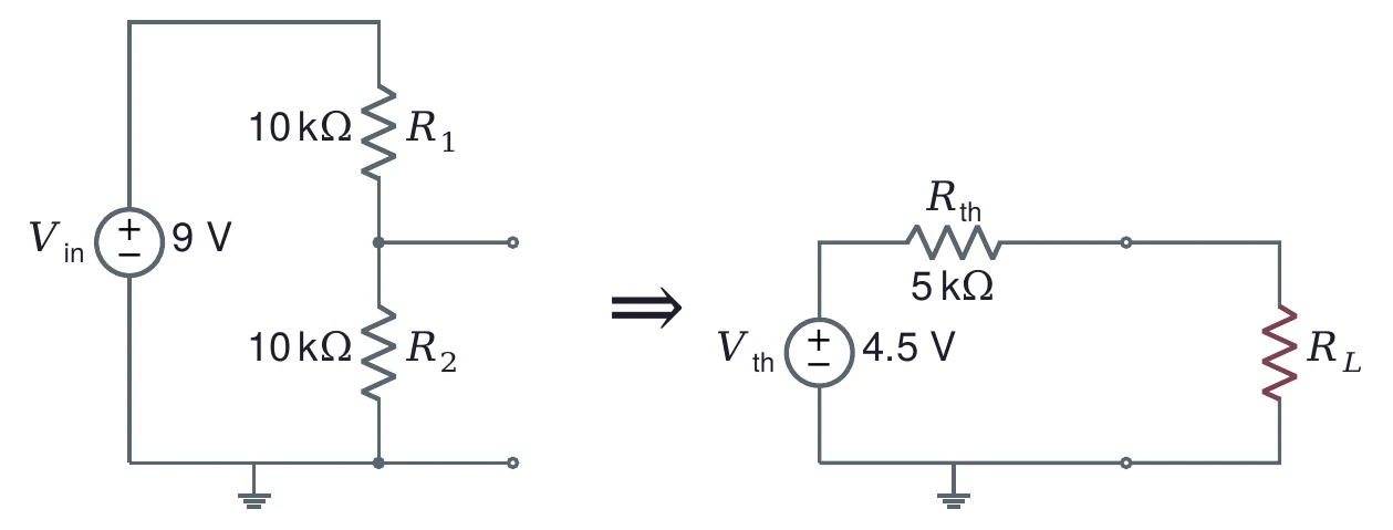
For the two 10 kΩ resistors, = 4.5 V and = 5 kΩ. Equation (2) with gives the same answers as Equation (5), and the firm rule says the divider is firm for loads above 50 kΩ. That is the design rule for a divider that must feed a load: make at least ten times smaller than the load. Lab 2 shows that every circuit of sources and resistors can be reduced this way. That is Thévenin's theorem.
6.3 Even the DMM is a load
A voltmeter must draw a little current to measure, so it is a load too. Many DMMs have about 10 MΩ of input resistance on their DC voltage ranges; your meter's manual gives its value. Against kilohm resistors, 10 MΩ changes nothing you can see. Against megohm resistors, it does.
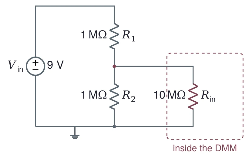
Unloaded, the output is 4.50 V. The meter puts 10 MΩ in parallel with the lower 1 MΩ: 1 MΩ ∥ 10 MΩ = 0.909 MΩ. The meter reads = 4.29 V, 4.8 % low. The circuit is fine; the measurement changed it.
(a) A divider of two 4.7 kΩ resistors runs from 10 V. Find and the loading effect for a 47 kΩ load.
(b) Find and for that divider, and use Equation (2) to check your answer to (a).
(c) A divider of two 470 kΩ resistors runs from 10 V. What does a 10 MΩ meter read across the lower one? How could you change the divider so the meter's error drops below 1 %?
7 The Oscilloscope
7.1 Three groups of controls
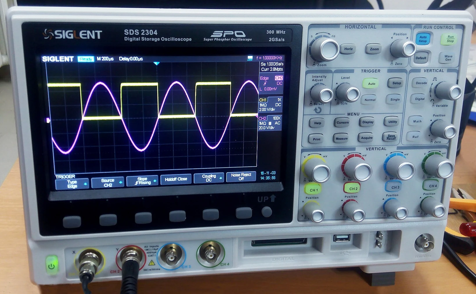
An oscilloscope draws voltage against time. Its screen is a grid, usually 10 divisions across and 8 high. The controls come in three groups. The vertical controls set volts per division for each channel. The horizontal control sets time per division for all channels. The trigger decides when each sweep across the screen starts.

7.2 Triggering
The scope redraws the screen many times a second. If each sweep starts at a random point of the waveform, the sweeps land on top of each other out of step and the screen shows a blur. The trigger fixes this. It waits until the signal crosses a set level in a set direction, then starts the sweep. Every sweep then starts at the same point of the waveform and the trace stands still.
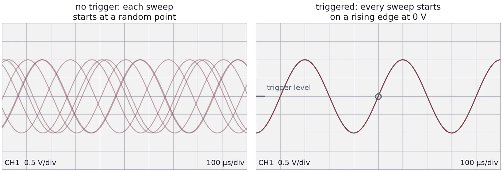
For a stable trace, set the trigger source to the channel you are measuring, the slope to rising, and the level somewhere inside the signal. A level above the top of the signal never triggers. Use edge triggering in Normal or Auto mode; Auto keeps drawing even when no trigger comes, which helps you find a signal.
7.3 Reading the screen
Count divisions, then multiply by the scale. In Figure 26, one period spans 4.0 divisions at 100 µs/div, so = 400 µs and = 2.50 kHz. Peak to peak spans 4.0 divisions at 0.5 V/div, so = 2.0 V. The amplitude is half of that, 1.0 V, and for a sine the RMS value is the amplitude divided by , 0.71 V.
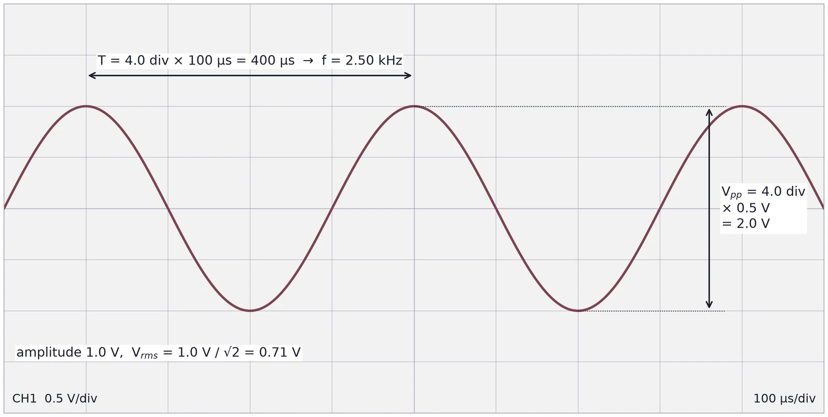
Choose the scales so the signal fills most of the screen: several periods across, and most of the height. Reading is more precise when the thing you read spans more divisions. The scope's built-in measurements and cursors read the same quantities with finer resolution; say in your report which you used.
7.4 Period and frequency errors
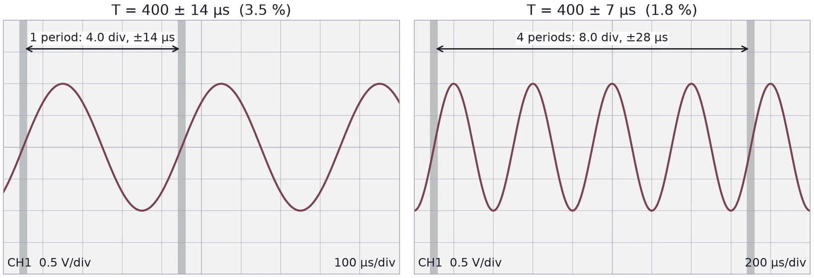
Suppose you can place each zero crossing to ±0.1 division, which is ±10 µs at 100 µs/div. A period is the difference of two crossings, so their errors combine:
Since , the relative error of the frequency is the same 3.5 %, but its absolute error is in hertz: = 0.035 × 2500 Hz = 88 Hz, so = 2.50 ± 0.09 kHz. Keep the two apart in your report: in microseconds, in hertz.
Measure across several periods and divide, and the reading error is shared among them. To fit four periods (1.6 ms) on the screen you need 200 µs/div, where ±0.1 division is ±20 µs. The four periods then carry ±28 µs, which is ±7 µs per period, 1.8 %: half the error of reading one period.
7.5 Two settings to check
| Setting | If it is wrong |
|---|---|
| Probe factor on the scope channel (1× or 10×) | Every voltage is 10 times too large or too small |
| Generator load setting (50 Ω or High-Z, §4.4) | The scope shows twice the amplitude the generator displays |
A 10× probe divides the signal by ten and presents about 10 MΩ to the circuit instead of 1 MΩ. The scope only knows to multiply back by ten if the channel's probe setting says 10×. A plain BNC cable from the generator is a 1× connection.
7.6 Export the data, then plot it
A digital scope can save the trace as a CSV file on a USB drive: one column of time and one column of voltage per channel, after a few header lines that differ from scope to scope. Open the file, check the units in the header, and plot voltage against time.
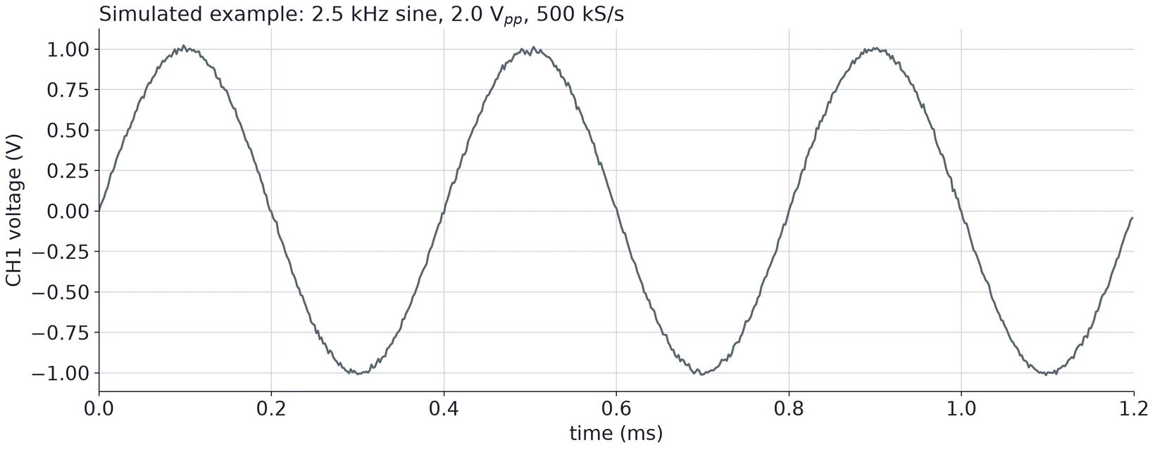
A good report plot has labeled axes with units, a scale that suits the numbers (milliseconds rather than 0.0012 s), a title or caption that says what was measured, and a source note if the data are simulated.
(a) On a screen at 200 µs/div and 2 V/div, one period of a sine spans 5.0 divisions and the trace spans 3.2 divisions from top to bottom. Find , , and .
(b) If you can read each crossing to ±0.1 division, what are and for (a)?
(c) The generator says 2.0 Vpp and the scope reads 4.0 Vpp. Name two settings that could explain it.
8 Error Analysis
Every task in this course needs an error analysis. For each value you report, state its uncertainty, name the main sources of error, and compare it with the value you expected, simulated or took from a datasheet.
| Measurement | Main error sources |
|---|---|
| Resistance | DMM specification for the range; lead resistance for small values; your body in parallel for large ones |
| Divider voltage | Resistor tolerance and rounding; the supply's set voltage; the meter's input resistance |
| Loading effect | The errors of the two voltages it is computed from |
| Period, frequency, amplitude | Reading the grid or cursors; trace thickness and noise; the scope's own accuracy; probe and generator settings |
A difference between measured and expected is only meaningful when it is larger than the uncertainty. When it is, say which source most likely explains it, and check that the size fits.