1 Where Lab 2 Sits
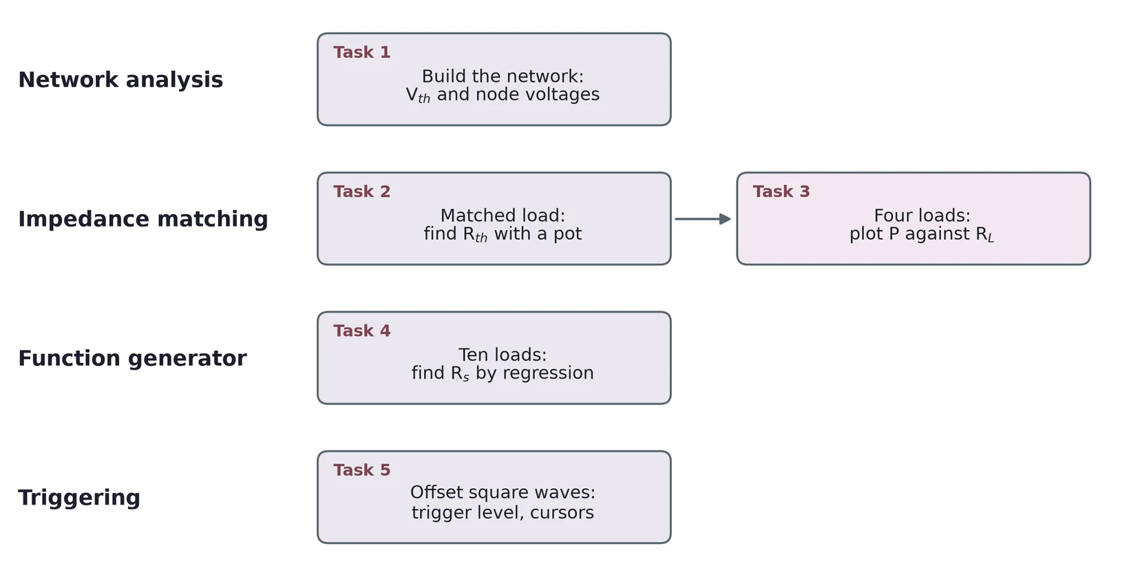
Lab 1 ended with a surprise: seen from its output, a voltage divider behaves like a source with a resistance inside. Lab 2 shows that every network of sources and resistors does the same. You reduce a network to one source and one resistor, then find that resistor on the bench in three ways. Last, you measure the resistance inside the function generator and learn to trigger on square waves that sit above 0 V.
1.1 Task map
| Lab 2 task | What you do | Concept & section |
|---|---|---|
| 1 | Build a network; find and the node voltages | Thévenin's theorem (§2), Kirchhoff's laws (§5) |
| 2 | Find with a 10 kΩ pot | The matched-load method (§4.5) |
| 3 | Four loads; plot power against | Maximum power transfer (§4) |
| 4 | Ten loads on the generator; find by regression | Impedance (§3), regression (§6) |
| 5 | Trigger on three square waves; read them with cursors | Triggering on offset waves (§7) |
Every task needs an error analysis. Section 8 collects the main error sources for each kind of measurement.
2 Thévenin's Theorem
2.1 One source and one resistor
Pick two terminals, A and B, in any circuit made of DC sources and linear resistors. Thévenin's theorem says that, seen from A and B, the whole circuit acts like one ideal source in series with one resistor . A load connected to A and B gets the same voltage and the same current from the real circuit as from the equivalent. The load cannot tell them apart.
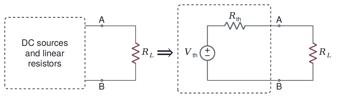
"Linear" matters. A resistor's current is proportional to its voltage, so every voltage in the network is a weighted sum of the sources, and the equivalent holds for every load. A diode or a transistor breaks this, and Lectures 04 and later deal with them.
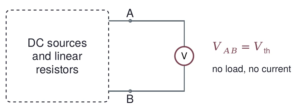
The first number is easy to measure. Remove the load and measure the voltage across A and B. With no load there is no current through , so nothing drops across it, and the voltmeter reads :
2.2 Zeroing sources and finding Rth
is the resistance you see looking into A and B when every source in the network is turned off. "Turned off" means set to zero, and the two kinds of source zero differently:
A voltage source set to 0 V keeps both ends at the same voltage for any current. That is a wire: replace it with a short.
A current source set to 0 A lets no current through for any voltage. That is a break: replace it with an open.
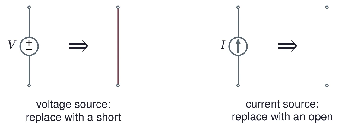
With the sources zeroed and the load removed, combine the resistors seen from A and B in series and parallel. The result is , the resistance between the load terminals with the load open. On the bench you cannot always zero a source, so Section 4 shows ways to find with the sources on.
2.3 A worked example
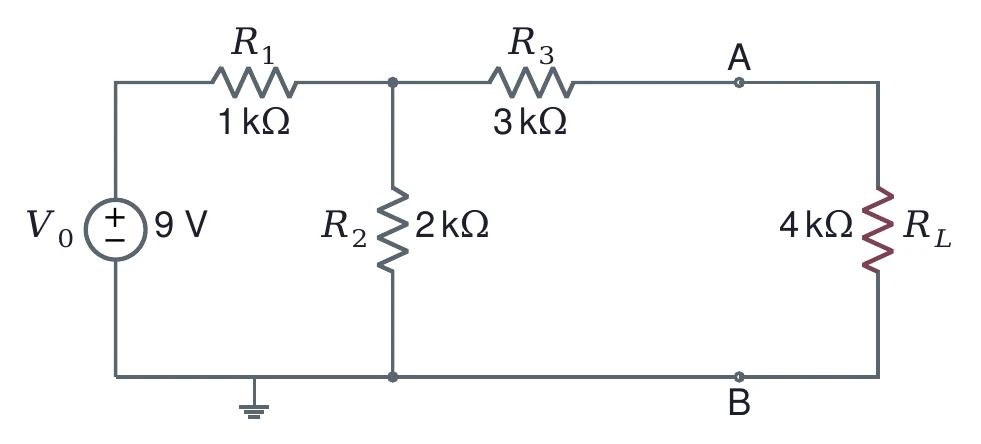
Figure 5 is the example from the lecture: a 9 V source, = 1 kΩ in series, = 2 kΩ to ground, and = 3 kΩ to terminal A. The load is = 4 kΩ. We want , and the load current .
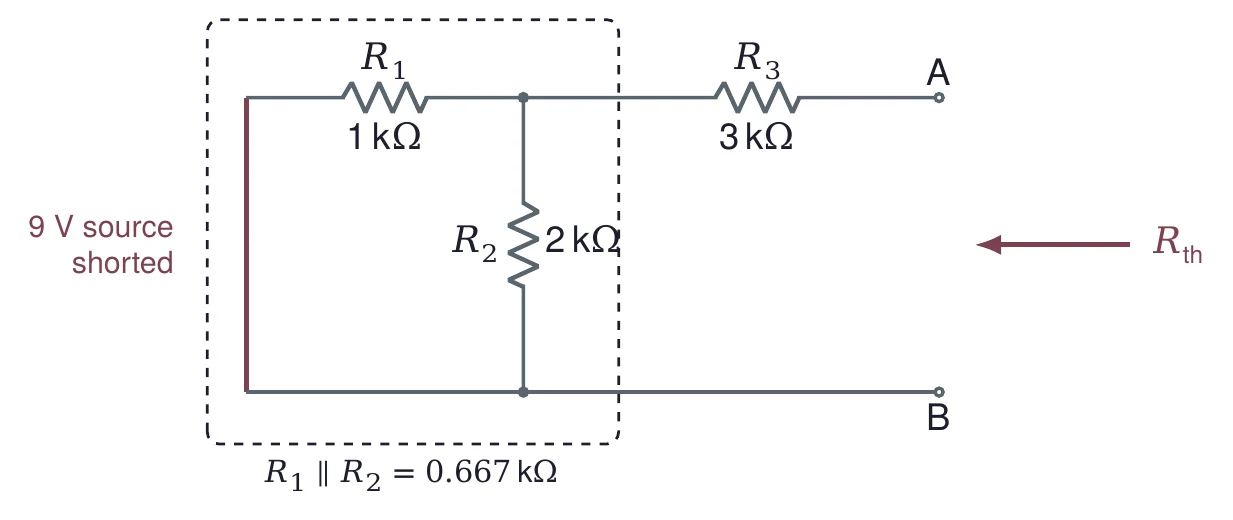
Remove the load and replace the 9 V source with a short (Figure 6). Looking in from A, you see in series with whatever is behind it. Behind it, now runs from the node to ground through the short, so and are in parallel:
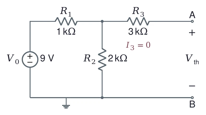
Put the source back and leave A and B open (Figure 7). No current flows into A, so none flows in and nothing drops across it. equals the voltage across , which is the output of a divider:
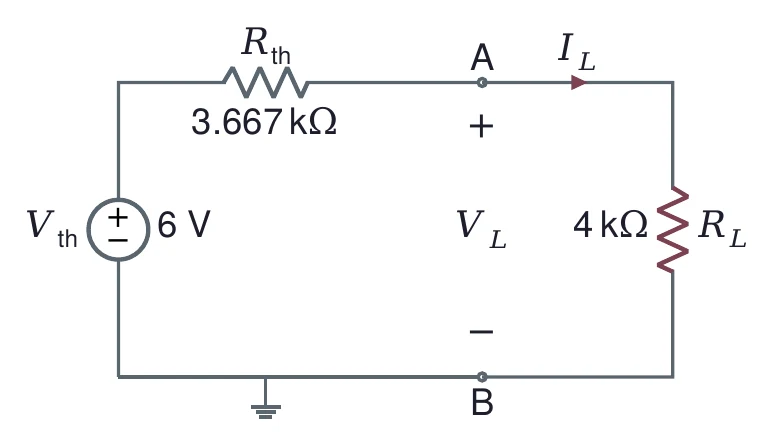
Connect the load to the equivalent (Figure 8). It is now a single loop, a divider of and :
Check it on the full circuit. The 9 V source sees in series with = 2 kΩ ∥ 7 kΩ = 1.556 kΩ, so = 9 V/2.556 kΩ = 3.522 mA. The node between and sits at 9 − 3.522 = 5.478 V, and the current through and is 5.478 V/7 kΩ = 0.783 mA. Same answer.
2.4 One equivalent, every load
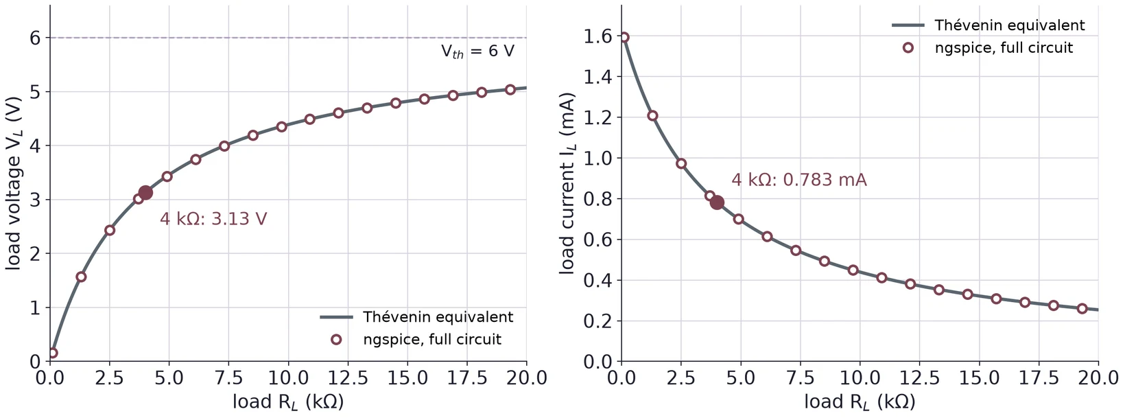
The work of finding and is done once. After that, any load is a one-line divider. Figure 9 sweeps the load from 100 Ω to 20 kΩ. The curves come from the equivalent; the circles come from an ngspice simulation of the full four-resistor circuit with swept. They agree at every point. As grows, climbs toward = 6 V and falls toward zero. With = 0 (a short), = 1.64 mA, the short-circuit current.
2.5 Ladders: reduce one stage at a time
A ladder alternates series and shunt resistors. You could write equations for every node, but Thévenin's theorem lets you walk along it. Cut the ladder after the first shunt resistor, replace everything to the left with its equivalent, and repeat.
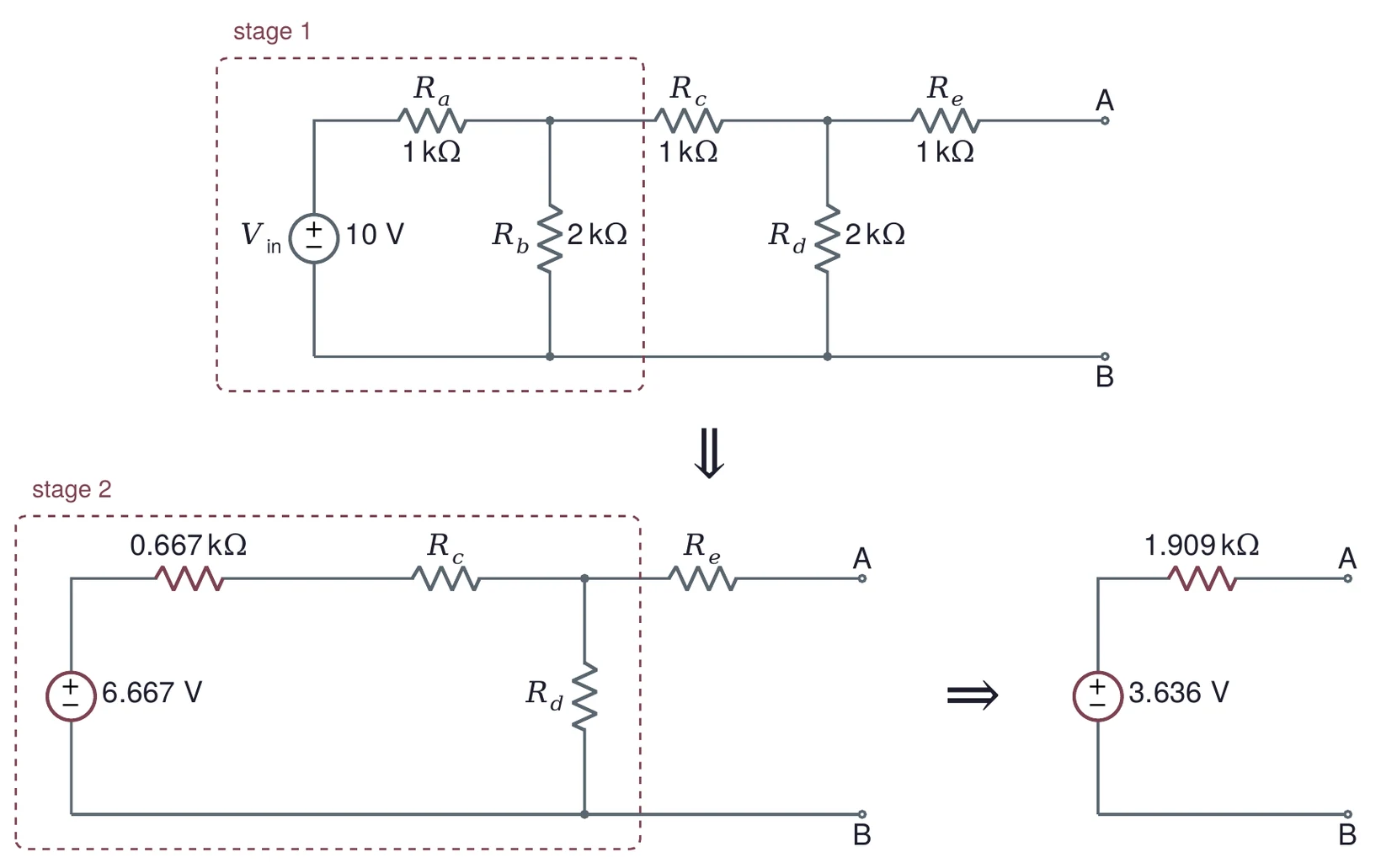
The ladder in Figure 10 runs from 10 V with = 1 kΩ in series, = 2 kΩ shunt, = 1 kΩ series, = 2 kΩ shunt and = 1 kΩ series to A.
Stage 1 (, , ) is a divider: = 6.667 V behind = 0.667 kΩ.
Stage 2 is that source, then in series and as the shunt. Its open voltage is = 3.636 V, and its resistance is = 0.909 kΩ.
adds in series: = 3.636 V and = 0.909 + 1 = 1.909 kΩ.
(a) A 12 V source feeds = 4.7 kΩ in series, = 10 kΩ to ground, and = 2.2 kΩ to terminal A (the shape of Figure 5). Find and , then and for a 6.8 kΩ load.
(b) A 2 mA current source sits in parallel with a 3 kΩ resistor, and A and B are across both. Find and .
(c) Reduce a ladder of five 2.2 kΩ resistors (series, shunt, series, shunt, series) from 15 V. Which node voltages could you check with a DMM on the bench?
3 Impedance, Input and Output
3.1 Impedance extends resistance
Resistance is the ratio of voltage to current for a resistor. Capacitors and inductors also limit current, but their current is shifted in time against their voltage. Impedance keeps track of both the size and the shift by using a complex number:
is the resistance, the real part, and is the reactance, the imaginary part. Both are in ohms. Engineers write for , because is taken by current. A resistor has = 0. A capacitor has , and an inductor has , with .
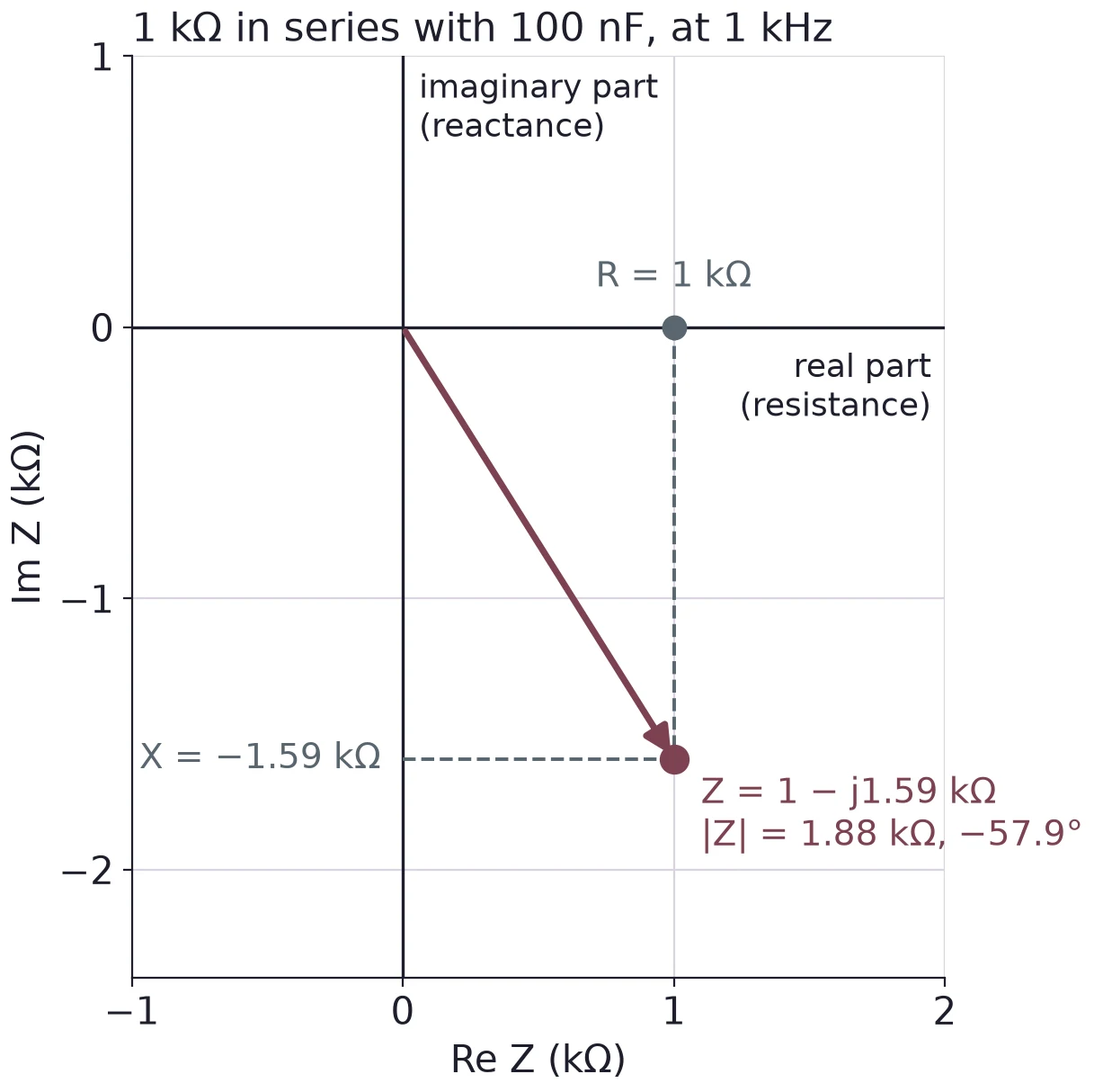
Series impedances add, as resistances do. In Figure 11 the capacitor's reactance at 1 kHz is = −1.59 kΩ, so the pair has = 1 − j1.59 kΩ. Its size is = 1.88 kΩ, the ratio of the voltage amplitude to the current amplitude.
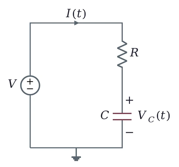
With a capacitor in the circuit, voltages and currents change with time, and Lecture 03 treats them properly. For this lecture one idea is enough: every source and every load has an impedance, and the divider rule works for impedances as it does for resistors.
3.2 Output impedance meets input impedance
Electronics is built from stages. A sensor drives an amplifier, the amplifier drives a filter, the filter drives a scope. Each stage's output is a source, and Thévenin's theorem says it looks like behind an output impedance . Each stage's input is a load with an input impedance . Where they meet, they form a divider:
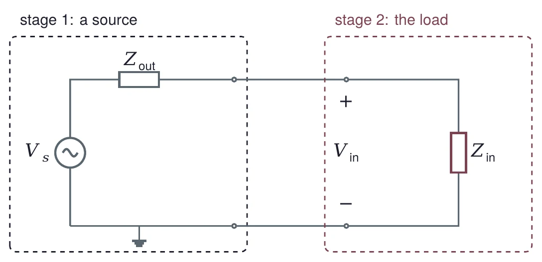
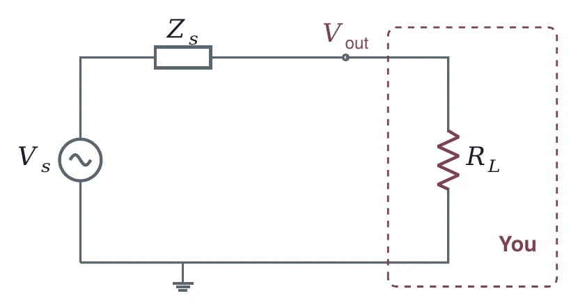
In the lecture's drawing, you are the load. Whatever you connect to a source, a DMM, a scope or the next stage, takes its share of , and the rest is lost across :
3.3 Bridging
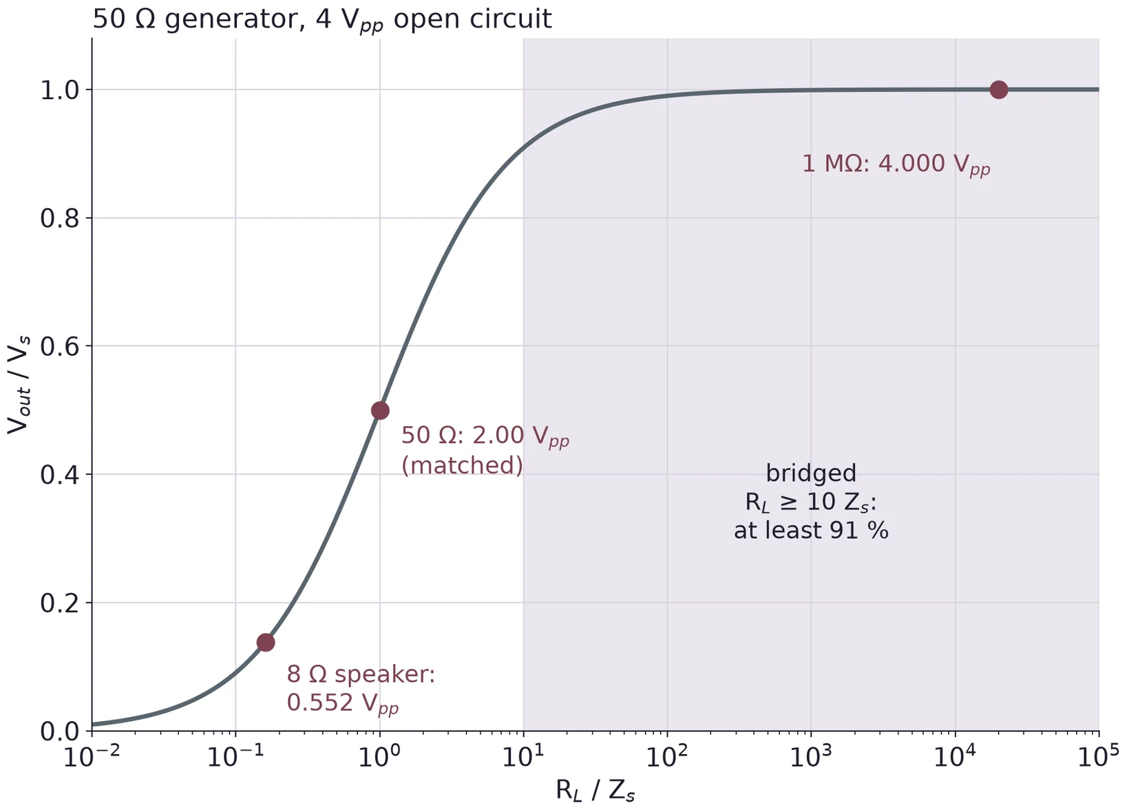
When the goal is to pass a voltage along, make large compared with . This is called bridging. The rule of thumb is the firm rule from Lecture 01: with , the load gets at least = 91 % of .
A generator with a 50 Ω output impedance is set for 4 Vpp open circuit.
Into a 1 MΩ scope input: = 3.9998 Vpp. Bridged; the scope sees the full voltage.
Into 50 Ω: = 2.00 Vpp. Matched; exactly half.
Into an 8 Ω speaker: = 0.552 Vpp, which is 0.1951 Vrms and = 4.76 mW. A generator is a poor speaker driver.
(a) A source with = 600 Ω gives 1.0 Vpp open circuit. What does it give into 10 kΩ, 600 Ω and 60 Ω? Which loads are bridged?
(b) A sensor has an output impedance of 2 kΩ. Is it bridged by a scope's 1 MΩ input? By an amplifier with = 10 kΩ? What fraction of its voltage reaches each?
(c) Find the real part, the imaginary part and for 2.2 kΩ in series with 47 nF at 2 kHz.
4 Maximum Power Transfer
4.1 Power in the load
The power a load takes is the product of its current and its voltage, . With Ohm's law it has two more forms:
For the example of §2.3 with the 4 kΩ load (Figure 8), = 0.783 mA × 3.130 V = 2.45 mW. That is far below the 0.4 W rating of the metal film resistors in Lecture 01's datasheet, so nothing warms up. The question the lecture asks next: is there a load that gets more?
4.2 Power peaks at RL = Rth
A small load takes a large current but has little voltage across it. A large load has nearly all of but takes little current. Somewhere between, the product peaks. Write the power with the divider of §2.3:
Set its derivative to zero:
The derivative is positive below and negative above it, so the peak is at . Put that back into Equation (6):
This is the maximum power transfer theorem, and a load with is matched.
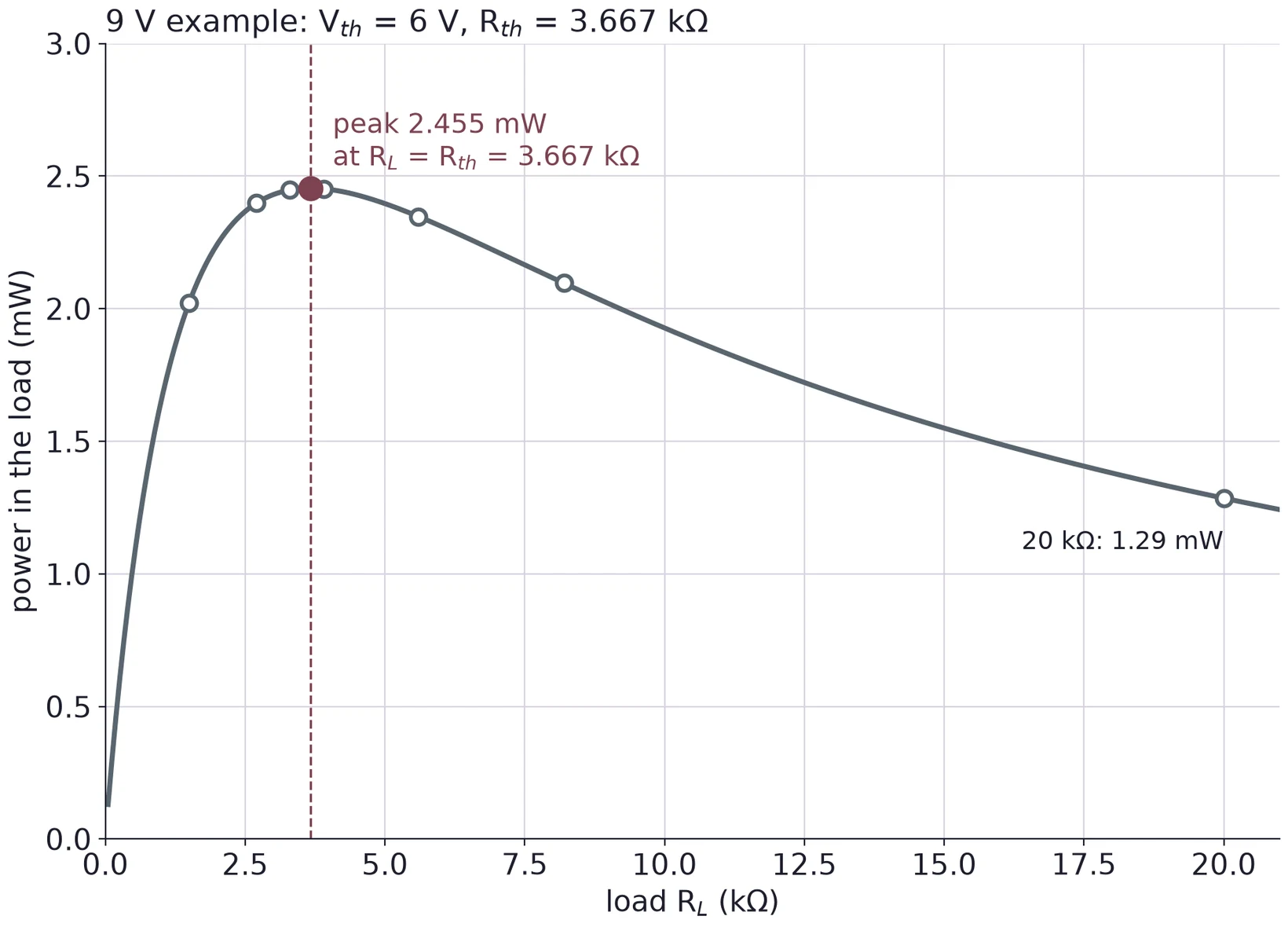
= 2.455 mW at 3.667 kΩ, with = 3.00 V. Seven standard values around it give:
| 1.5 kΩ | 2.7 kΩ | 3.3 kΩ | 3.9 kΩ | 5.6 kΩ | 8.2 kΩ | 20 kΩ | |
|---|---|---|---|---|---|---|---|
| (V) | 1.742 | 2.545 | 2.842 | 3.093 | 3.626 | 4.146 | 5.070 |
| (mW) | 2.023 | 2.398 | 2.448 | 2.452 | 2.348 | 2.096 | 1.285 |
The peak is flat: 3.3 kΩ and 3.9 kΩ both get within 0.3 % of the maximum.
4.3 Matched is not efficient
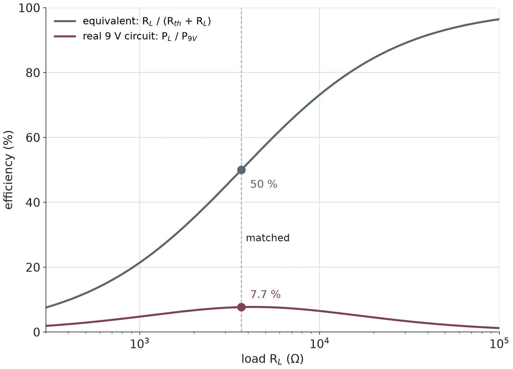
At the match, half of the power the equivalent source makes goes to the load and half heats . The equivalent's efficiency, , is 50 %. Equivalent source power is = 6 V × 0.818 mA = 4.91 mW.
The real circuit does worse. With the 3.667 kΩ load in Figure 5, the 9 V source supplies 3.545 mA, which is 31.91 mW. The load still gets 2.455 mW, only 7.7 %. Most of the rest heats (12.57 mW) and (14.88 mW), and 2.01 mW heats .
and give the right voltage and current for the load. They say nothing about the power inside the network. Use the real circuit to find the power the source supplies.
4.4 Match or bridge?
Matching gives the most power to the load; bridging passes the voltage along and wastes less. Which one a design wants depends on the job.
| Where | Choice | Why |
|---|---|---|
| RF circuits, antennas, 50 Ω coax | Matched | Signals are weak, so every bit of power counts, and a matched line sends no reflections back |
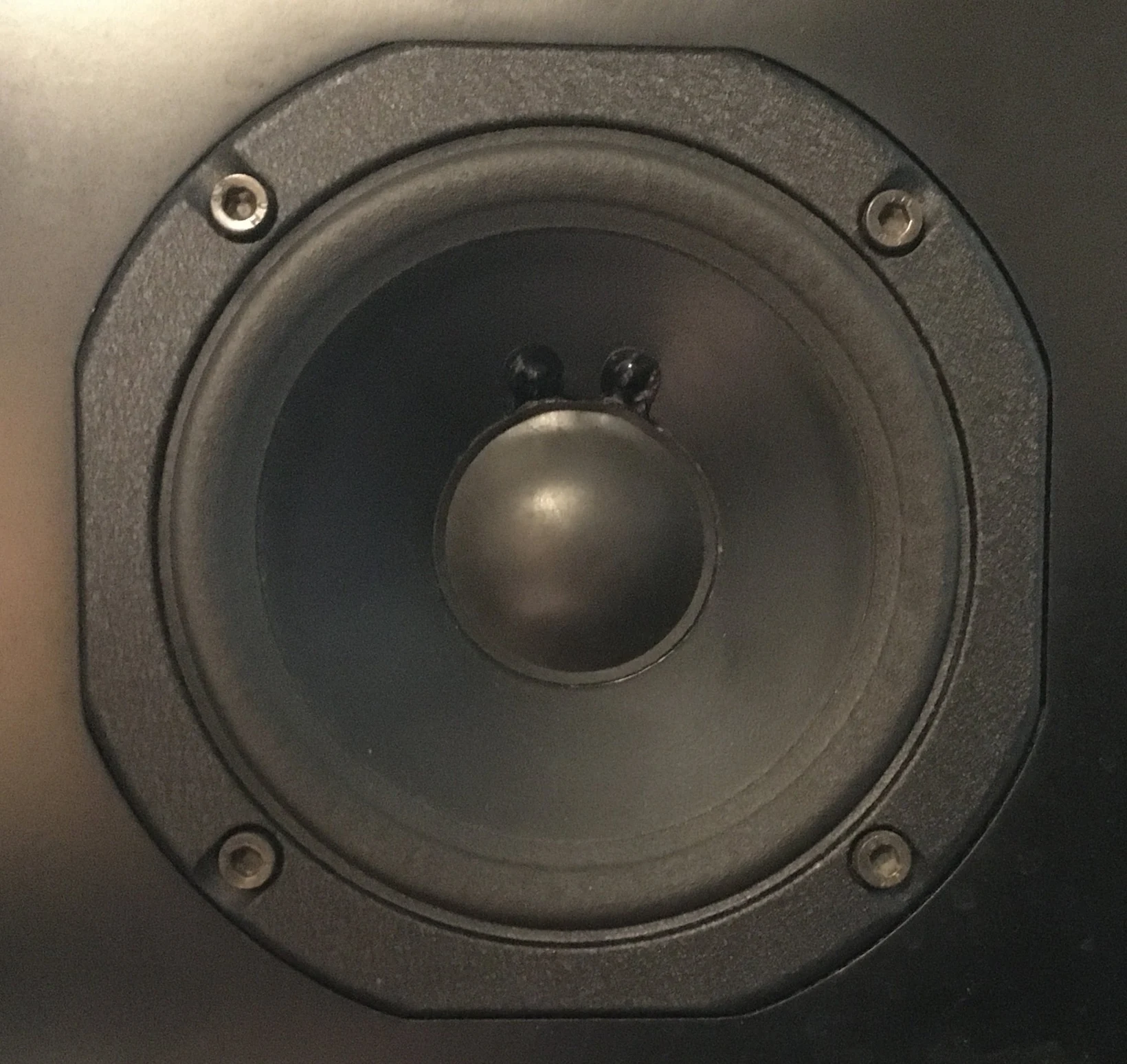
| Audio amplifier to speaker | Bridged | The amplifier's output impedance is far below the speaker's 8 Ω, so little power heats the amplifier |
| Power grid | Bridged | A matched grid would waste half of all the power it makes |
| Scope and DMM inputs | Bridged | An instrument should read the voltage, not change it |

4.5 The matched-load method
At the match, , so the load voltage is exactly half of . That gives a way to find with the sources on:
- Measure with nothing connected to A and B.
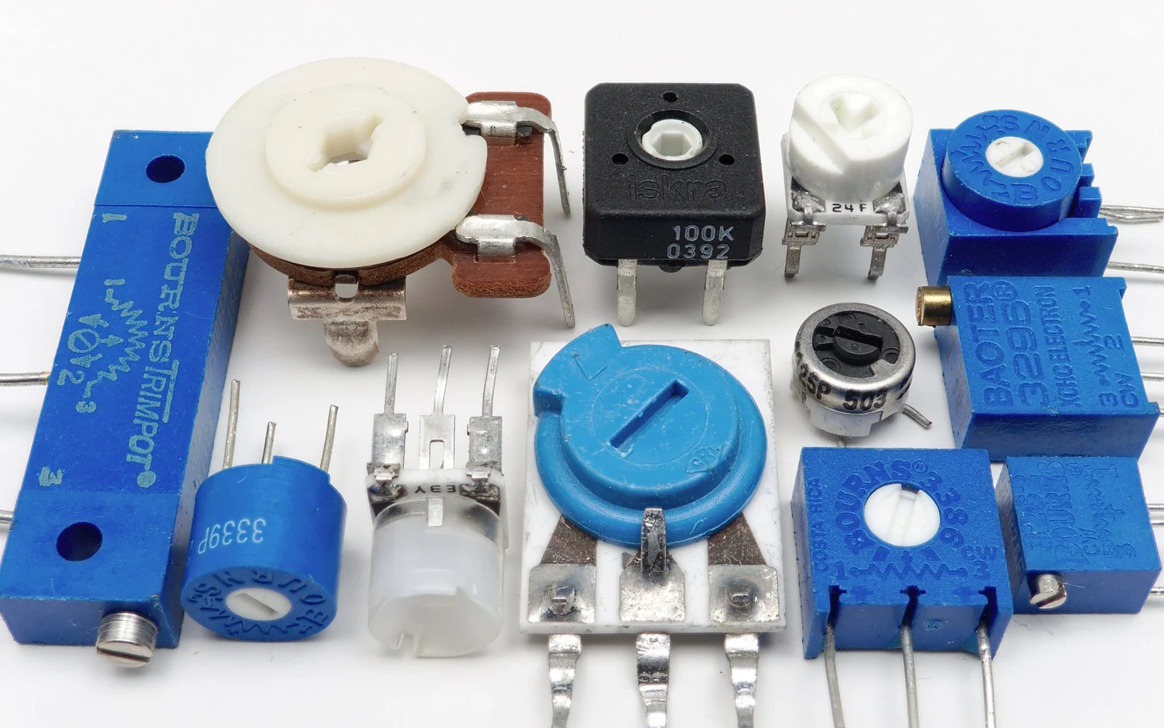
- Connect a potentiometer as , wired as a variable resistor (the wiper and one end).
- Turn it until the DMM across it reads .
- Disconnect the pot without touching the knob, and measure its resistance with the DMM, unpowered. That reading is .
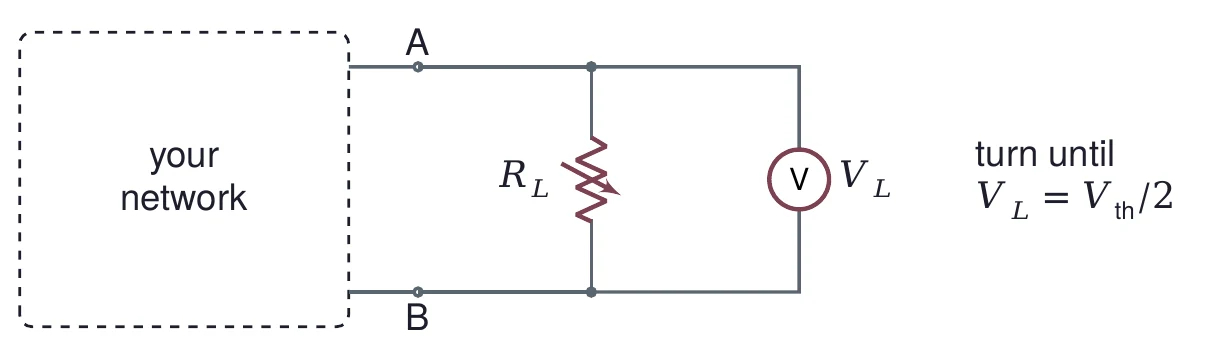
For the 9 V example you stop at 3.00 V, and the pot is then at 3.667 kΩ. The pot's own range must include .

How exact is the match? Write , so . Suppose you stop where the meter reads a fraction high, . Solving for :
With = 1 %, = 1.01/0.99 = 1.020, a 2 % error. For the 9 V example, readings from 2.97 to 3.03 V put the pot anywhere from 3.594 to 3.741 kΩ.
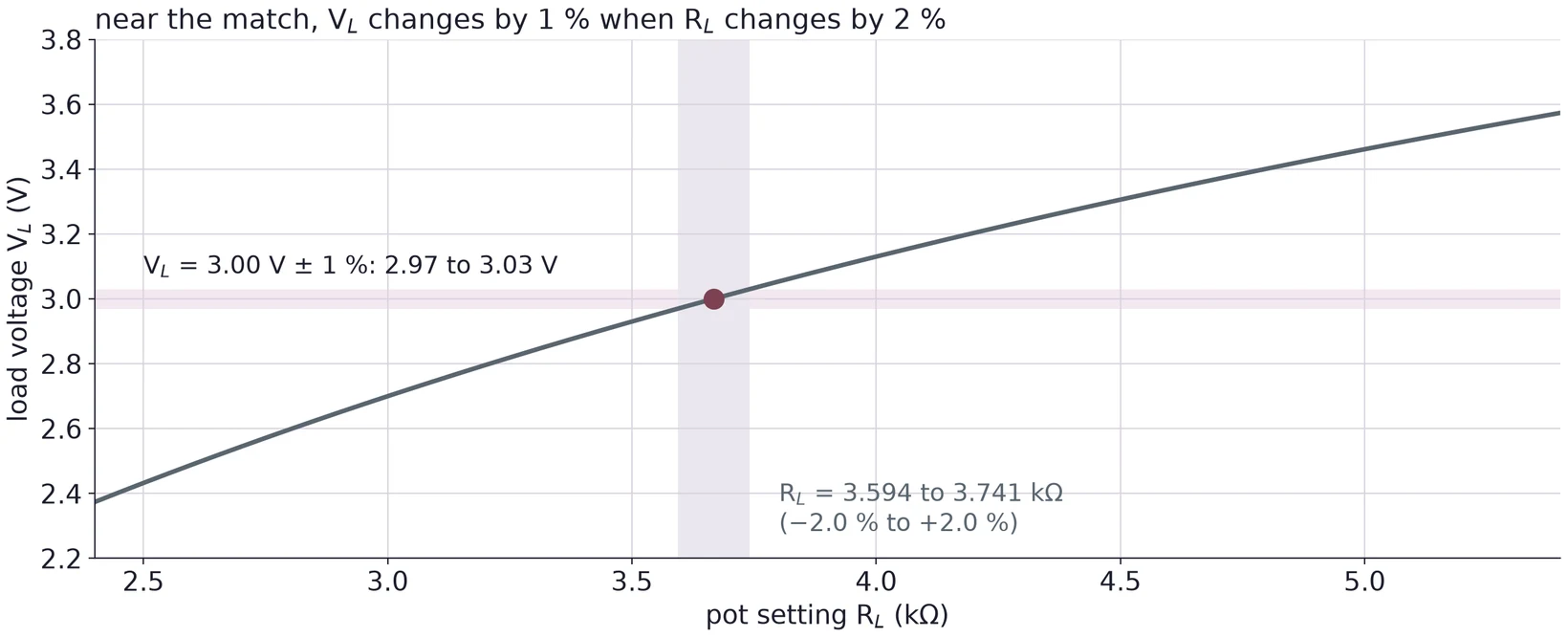
The slope of against is small at the match, so the voltage error doubles in the resistance. That is the price of a method that needs no current measurement.
4.6 The known-load method
You do not need a pot. Any known resistor works: measure open, connect a known , and measure . The divider solves for :
On the 9 V example, an 8.2 kΩ load gives = 4.146 V. Then = 3.667 kΩ.
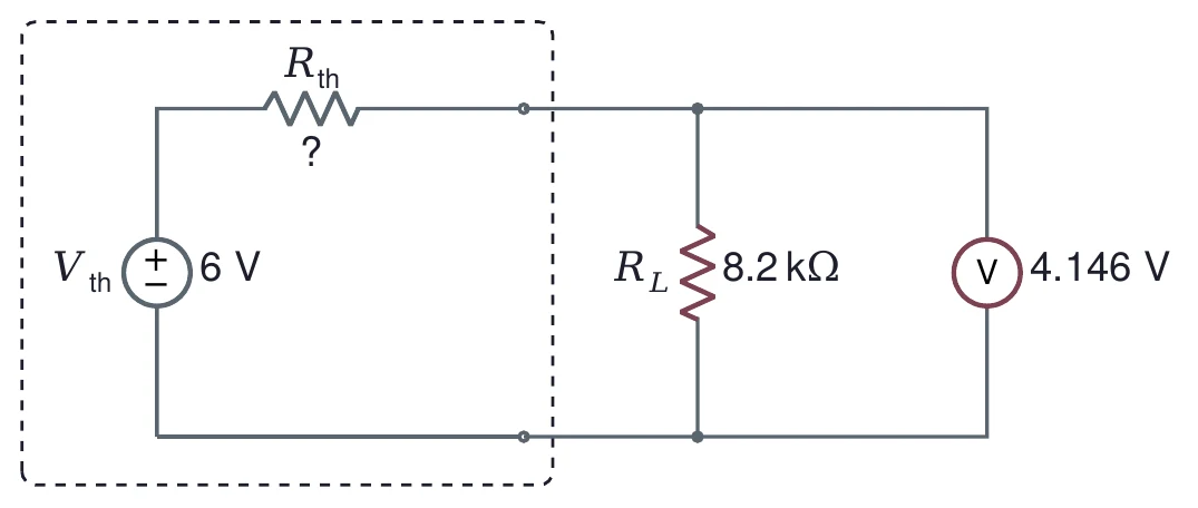
The same error rule holds here: a load near gives the best result, because there changes most for a change in .
(a) A network has = 4 V and = 1.2 kΩ. Find . Find the power in 820 Ω and in 1.8 kΩ loads.
(b) For the network in (a), find the equivalent's efficiency at the match and at . How much power does each load get?
(c) In a matched-load measurement you stop where the meter reads 2 % above . How far is the pot from ?
(d) A network reads 4.20 V open and 3.50 V with a 10 kΩ load. Find . If each reading is uncertain by ±0.01 V, roughly how uncertain is ?
5 Kirchhoff's Laws and a Matrix
Thévenin's theorem answers questions about one pair of terminals. To find every current in a network at once, write Kirchhoff's laws and solve them together.
Kirchhoff's current law (KCL): the currents into a node add up to the currents out of it. Charge does not pile up in a wire.
Kirchhoff's voltage law (KVL): the voltage changes around any closed loop add up to zero.
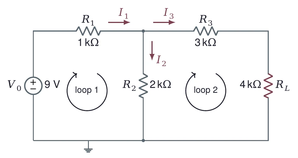
For the example circuit with the 4 kΩ load, take through , down and through and . One KCL equation at the top node and one KVL equation around each loop give three equations:
Move every unknown to the left and write them as a matrix equation :
numpy solves it in one call:
import numpy as np
R = np.array([[1,    -1,   -1],
              [1e3,  2e3,  0],
              [0,   -2e3,  7e3]])
V = np.array([0, 9, 0])
I = np.linalg.solve(R, V)
print(I * 1e3)          # in mA
Example only. Do not copy this code as it is: read it, learn from it, then write your own.
[3.52173913 2.73913043 0.7826087 ]= 3.522 mA, = 2.739 mA and = 0.783 mA, the same load current as the Thévenin equivalent in §2.3. KCL checks: 2.739 + 0.783 = 3.522.
The loops give a smaller system. Let a mesh current circle loop 1 and circle loop 2, both clockwise. carries . KVL around each loop gives
and np.linalg.solve returns = 3.522 mA and = 0.783 mA, which are and . Two unknowns instead of three: mesh currents satisfy KCL by construction.
The matrix method and Thévenin's theorem answer different questions. The matrix gives every current for one load. The equivalent gives the load current for every load. For a network like Lab 2's, with many nodes to record, the matrix (or a SPICE simulation, which solves the same equations) is a good check on your hand calculation.
(a) For a 12 V source with = 2.2 kΩ, = 4.7 kΩ, = 1 kΩ and = 3.3 kΩ in the shape of Figure 23, write the 3 × 3 matrix equation and the 2 × 2 mesh equation. Solve both with numpy.
(b) Find and for the same circuit and check that the equivalent gives the same .
(c) What changes in the matrix if is removed (an open)? What if it is shorted?
6 Measuring a Source's Resistance
6.1 Many loads, one line
A function generator is a source with a resistance inside (Lecture 01, §4.4). To measure that resistance, , connect a load, read on the scope, and repeat with other loads. Each reading obeys the divider:
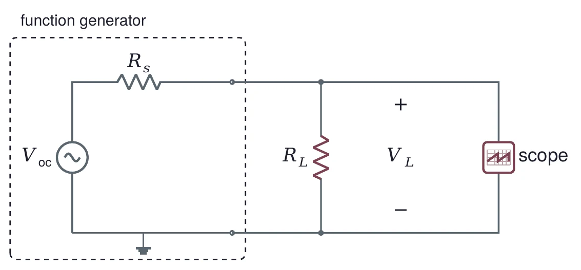
A plot of against is a curve (Figure 25, left), and a straight-line fit through it means nothing. Rewrite Equation (11) with the load current and it becomes a line:
Plot against . The slope is and the intercept is . A second way: take the reciprocal of Equation (11), , and fit against .
A simulated source has = 3.00 Vpp and = 100 Ω. Ten loads from 22 to 680 Ω give these readings, rounded to 10 mV as a scope might:
| (Ω) | 22 | 33 | 47 | 68 | 100 | 150 | 220 | 330 | 470 | 680 |
|---|---|---|---|---|---|---|---|---|---|---|
| (Vpp) | 0.54 | 0.74 | 0.96 | 1.21 | 1.50 | 1.80 | 2.06 | 2.30 | 2.47 | 2.62 |
A least-squares line through (, ) gives a slope of −100.4 ± 0.3 Ω and an intercept of 3.002 Vpp, so = 100.4 ± 0.3 Ω. Fitting against gives the same 100.4 Ω and 3.002 Vpp. The 0.4 Ω offset from the true 100 Ω comes from the rounding.
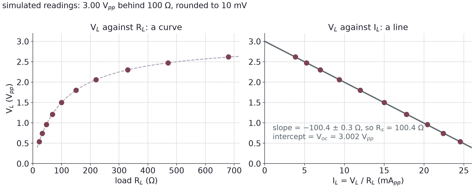
In numpy, p, cov = np.polyfit(I, V, 1, cov=True) returns the slope in p[0] and its variance in cov[0, 0]; the square root is the slope's standard error. Report with that uncertainty.
6.2 Choosing the loads
Which loads tell you the most? Use one load to see it. From Equation (11), . If reads 1 % high, the estimate is off by about percent.
For the simulated source above: with a 22 Ω load, the estimate is 98.8 Ω (−1.2 %). With 100 Ω, 98.0 Ω (−2.0 %). With 680 Ω, 92.3 Ω (−7.7 %).
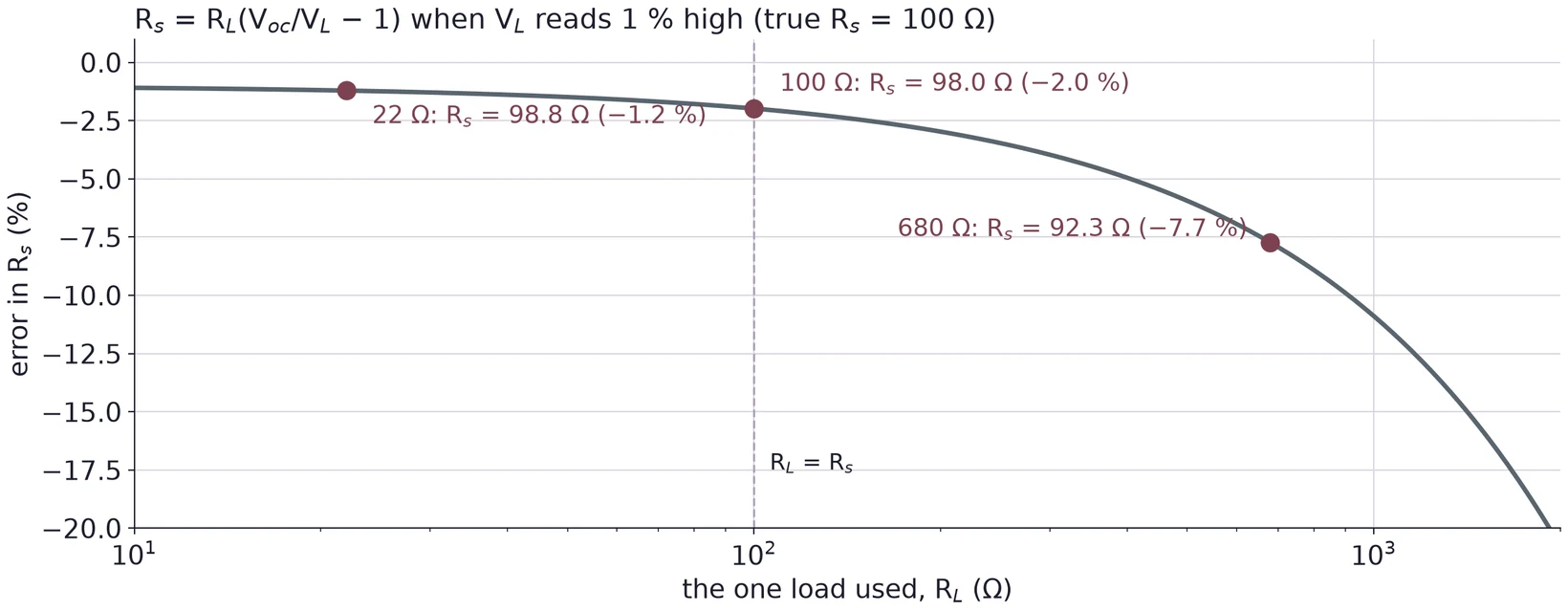
A load far above barely pulls the voltage down, so the small drop across is lost in the reading error. Loads near and below it tell you the most. The smallest loads have their own problem: gets small, and a fixed reading error of the scope is then a larger fraction of it. Spread the loads around , as the ten values above do around 100 Ω.
6.3 Check the generator's output setting
Many generators have an output-load setting, 50 Ω or High-Z, that changes only what the display shows (Lecture 01, §4.4). It does not change , but it changes the open-circuit voltage you get for the amplitude you set. Write down which setting you used. The fit gives , and you can check it against a reading with no load at all.
(a) A source reads 2.06 Vpp into 150 Ω and 1.57 Vpp into 47 Ω. Find and from these two readings.
(b) Why would ten loads between 10 kΩ and 100 kΩ be a poor choice for a source with near 50 Ω?
(c) A generator is set to 0.6 Vpp in 50 Ω mode. What open-circuit voltage should the fit return?
7 Triggering on Offset Square Waves
7.1 Offset moves the wave
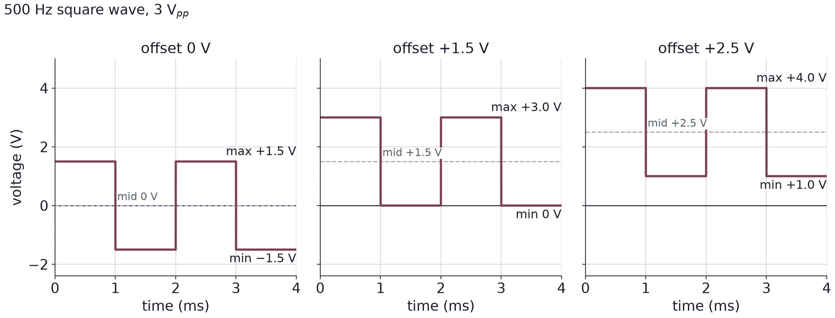
A function generator's offset adds a DC voltage to the wave. The shape and the peak-to-peak value stay the same; the whole wave moves up or down:
Offset 0: from −1.5 to +1.5 V, middle 0 V.
Offset +1.5 V: from 0 to +3.0 V, middle +1.5 V. The minimum sits at 0 V.
Offset +2.5 V: from +1.0 to +4.0 V, middle +2.5 V. The whole wave is above 0 V.
7.2 The trigger level and the coupling
The trigger starts each sweep when the signal crosses the trigger level (Lecture 01, §7.2). The level must lie between the minimum and the maximum, or the signal never crosses it. On a square wave the safest level is the middle, half way up the edge, where noise on the flat tops cannot cause a false trigger.
The input coupling decides what the scope sees. DC coupling shows the signal as it is, offset included. AC coupling puts a capacitor in series with the input, which blocks the average (DC) part: an offset square wave is shown centered on 0 V.
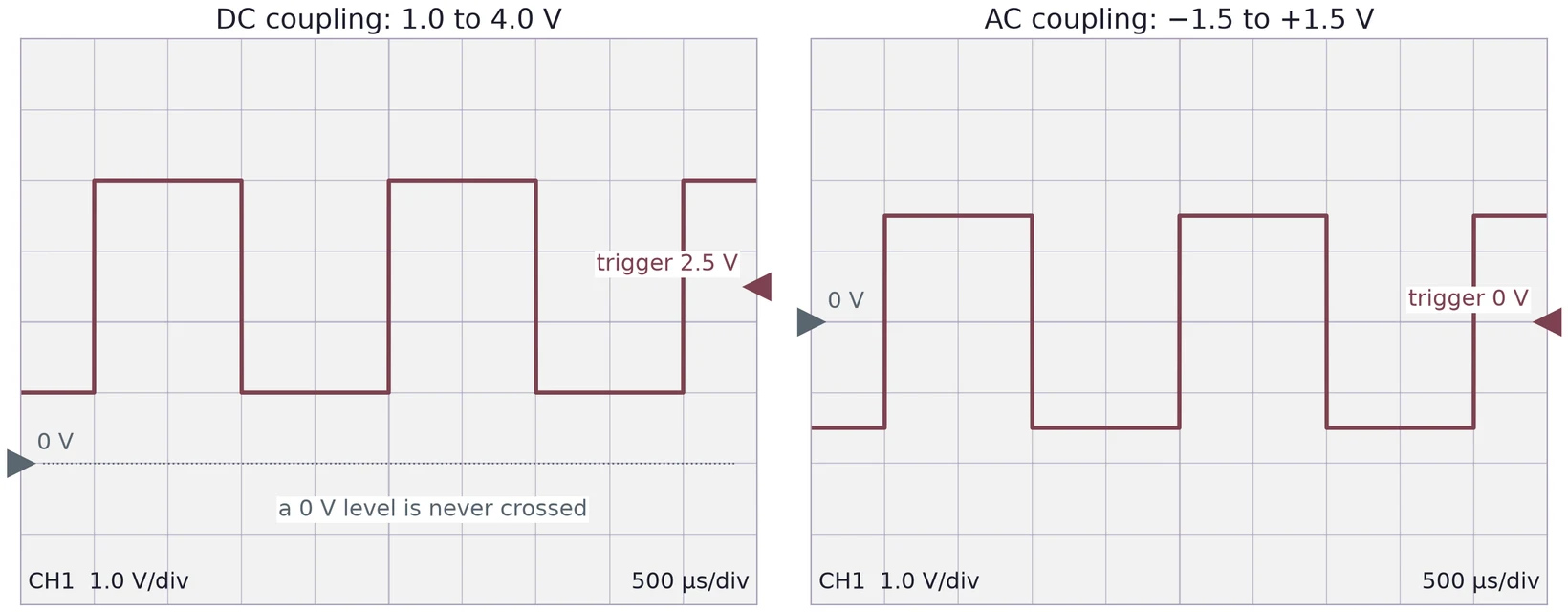
With DC coupling, the level must move with the offset. A level left at 0 V triggers on the first wave of the worked example, sits on the bottom edge of the second, and is never crossed by the third. In Auto mode the scope then draws untriggered sweeps, and the trace drifts. Use DC coupling when you need the real maximum and minimum, since AC coupling hides the offset. The ground marker at the left edge shows where 0 V is on the screen; move it down to make room for a wave above 0 V.
7.3 Cursors
Horizontal cursors are two lines you place on the screen; the scope prints the voltage of each and the difference between them. Put Y1 on the top of the wave and Y2 on the bottom. Then Y1 is the maximum, Y2 the minimum, and ΔY the peak-to-peak voltage.
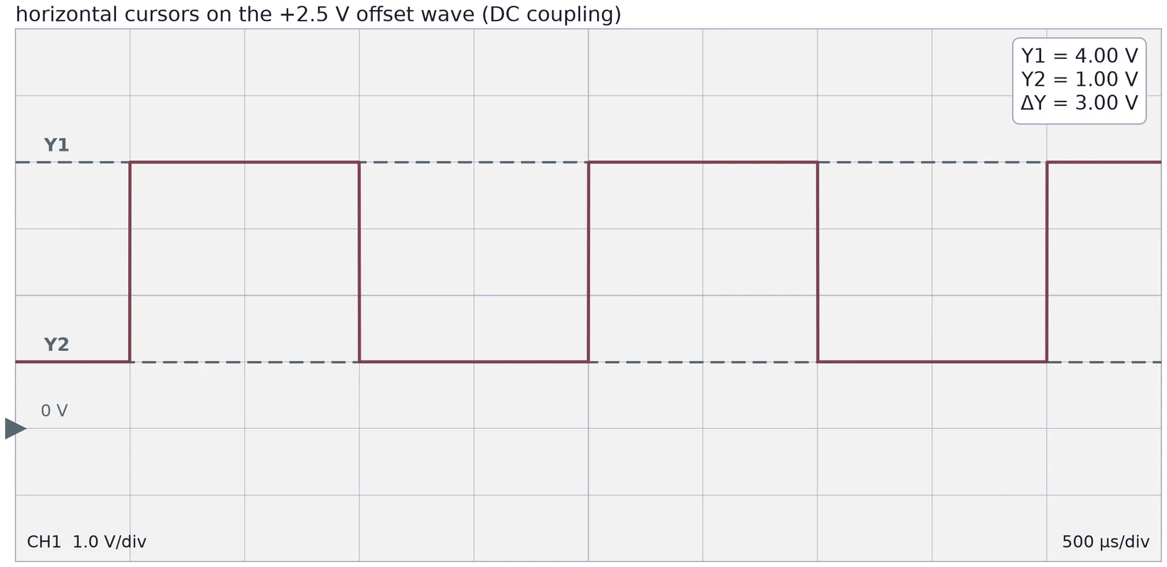
Cursor readings depend on the vertical scale. Choose a V/div that makes the wave fill most of the screen, and place each cursor in the middle of the trace's thickness. Some scopes also have automatic max, min and peak-to-peak measurements. Say in your report which you used.
(a) A 2 kHz square wave of 4 Vpp has a +3 V offset. Find its maximum, minimum and middle. Which trigger levels work in DC coupling?
(b) The same wave is viewed in AC coupling. Where are its top and bottom on the screen, and what trigger level works?
(c) You set a −0.5 V offset on a 1 Vpp square wave. What happens if you trigger at +0.2 V in DC coupling?
8 Error Analysis
Every task in this course needs an error analysis. For each value you report, state its uncertainty, name the main sources of error, and compare it with the value you expected, simulated or took from a datasheet.
| Result | Main error sources |
|---|---|
| Resistances | DMM specification for the range; lead resistance for small values |
| and node voltages | Resistor tolerance; the supply's set voltage; DMM accuracy |
| , matched load | Reading , which doubles in (§4.5); measuring the pot afterwards |
| Power against | The errors of and |
| by regression | The slope's standard error; scope reading; the choice of loads (§6.2); tolerance of the load resistors |
| Max, min, | Cursor placement; trace thickness and noise; the scope's vertical accuracy; coupling |
Comparing with your calculation. Recompute with the measured resistor values, not the nominal ones. A difference that remains is then due to the supply, the meter or the wiring, not the tolerance.
Power. uses twice, so its relative error counts twice. For independent errors,
With 1 % in and 1 % in , % = 2.2 %. For the 4 kΩ load of §2.3, = 2.45 ± 0.05 mW.
Matched-load and known-load results. Use Equation (8): a fractional error in the voltage at the match gives about in . Add the DMM's uncertainty for the pot reading.
Regression. Report the slope's standard error from the fit, and look at the residuals: points that curve away from the line point to a wrong load value or a reading error.
Cursor readings. Each cursor is placed to a fraction of a division. With ±0.1 division per cursor at 1 V/div, each of max and min is ±0.1 V, and is = ±0.14 V.
A difference between measured and expected is only meaningful when it is larger than the uncertainty. When it is, say which source most likely explains it, and check that the size fits.