Due: 2:00 p.m. before your next lab section.
- Report Format: Submit a typed lab report in PDF format. Hand-drawn circuit diagrams will not be accepted; draw every schematic with software (see Software at the end of this manual).
- Time: Plan your time. Makeup sessions are available by appointment with your TA, subject to their availability.
- AI Policy: The use of any AI tool, including a large language model (LLM), to write, generate, debug, or modify code or any portion of the lab report is prohibited unless the course instructor grants explicit permission in advance. A teaching assistant (TA) cannot grant permission to use AI tools.
By signing below, I acknowledge that I have read and understood the policies and instructions above and agree to follow them.
Student Name (print):
Student Signature: Date:
All tasks in this lab are required. The Lecture 02 notes cover Thévenin's theorem and the methods you need.
Network Analysis
Task 1: Network Construction and Analysis
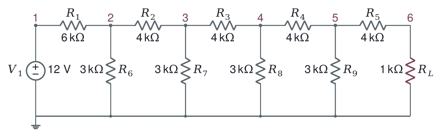
Build and analyze the network shown in Figure 1:
- Measure and record each resistor value before assembly.
- Find without measuring any current.
- Record the voltages at each numbered node (1 to 6).
- Compare your results with your homework calculations.
Course Instructor or TA Signature:
Date and Time:
Impedance Matching
Task 2: Matched-Load Method
Using your constructed network:
- Connect a 10 kΩ potentiometer as .
- Find using the matched-load method.
- Turn the power off, disconnect the potentiometer, and measure its resistance with the DMM.
- Compare this result with your Task 1 measurements.
- Document any discrepancies and their possible sources of error.
Course Instructor or TA Signature:
Date and Time:
Task 3: Load Variation Effects
Study the effect of different loads:
- Replace with a 4.7 kΩ resistor.
- Measure and calculate the power delivered.
- Test with additional loads: 1 kΩ, 2.2 kΩ and 10 kΩ.
- Plot power against load resistance.
- Identify the maximum power transfer point.
Course Instructor or TA Signature:
Date and Time:
Function Generator Characterization
Task 4: Source Impedance Measurement
Determine the function generator's output impedance:
- Set the generator to output a 1 kHz sine wave, 2 Vpp.
- Measure with 10 different loads (10 Ω to 330 Ω).
- Plot load voltage against load resistance.
- Plot load voltage against load current (). This plot is a straight line.
- Calculate from that line using linear regression.
- Save the data for your lab report.
Course Instructor or TA Signature:
Date and Time:
Triggering Practice
Task 5: Square Wave Analysis
Learn advanced triggering with square waves:
- Set the function generator for a 1 kHz square wave:
- Case 1: 2 Vpp centered at 0 V
- Case 2: 2 Vpp with its minimum at 0 V
- Case 3: 2 Vpp with a +1.5 V offset (minimum above 0 V)
- For each case:
- Set the proper trigger level for a stable display.
- Use cursors to measure the peak-to-peak voltage.
- Measure the maximum and minimum voltage levels.
- Save screenshots showing stable triggering for each case.
- Explain the difference in trigger level settings between the cases.
Course Instructor or TA Signature:
Date and Time:
Submission Reminder
- Task 1: the measured resistor values, , the six node voltages, and the comparison with your homework calculations.
- Task 2: your matched-load value of and its comparison with Task 1.
- Task 3: and the power for each load, the plot of power against load resistance, and the maximum power transfer point.
- Task 4: the table of loads and voltages, your two plots, and from the regression.
- Task 5: the screenshots, the maximum, minimum and peak-to-peak voltages for each case, and your explanation of the trigger levels.
- An error analysis for every task where it applies: the uncertainty of each measured or calculated value, its main sources of error, and a comparison with the expected, simulated, or datasheet value.
- A discussion of any challenges you met and how you solved them.
Draw every circuit diagram with software; hand-drawn circuit diagrams will not be accepted. We recommend the free draw.io; the course’s Drawing Circuit Diagrams page shows how to set it up. If a component has no symbol of its own, use the closest one and label it clearly.
Where a task asks for a simulation: the web version of Multisim is no longer available. If you have a Windows computer, you can install the offline (desktop) version of Multisim; ask a TA for the serial number to install it. Otherwise, feel free to use any SPICE-based simulation tool, such as LTspice or ngspice.