← All course materialsLecture 02 · Thévenin’s theorem & impedance matchingReading notes →

Lecture 02: Thévenin's Theorem and Impedance Matching

1 / 33
PHYS 252 · Lecture 0201

Lecture 02

Thévenin's Theorem and Impedance Matching

Part 1 · Thévenin's theorem · Part 2 · impedance · Part 3 · maximum power · Part 4 · Kirchhoff and a matrix · Part 5 · a real source · Part 6 · triggering

© Ran Yang, Ph.D.Electronics
PHYS 252 · Lecture 0202

Part 1 · Lab 2 in five tasks
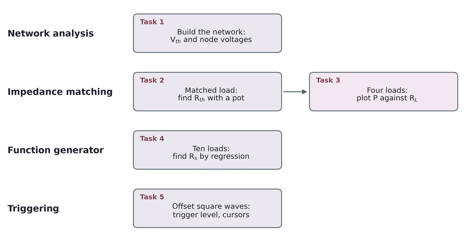
Lab 2 in four rows. Network analysis: Task 1, build the network and find V_th and the node voltages. Impedance matching: Task 2, the matched-load method with a pot to find R_th, then Task 3, four loads and a plot of power against load resistance. Function generator: Task 4, ten loads and a regression to find R_s. Triggering: Task 5, offset square waves, trigger level and cursors.

You reduce a network to one source and one resistor, then find that resistor three ways. Last, you measure the generator and trigger on offset waves.

© Ran Yang, Ph.D.Electronics
PHYS 252 · Lecture 0203

Any linear circuit looks like one source and one resistor
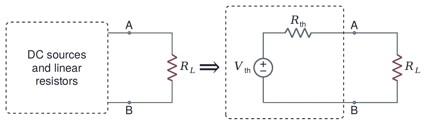
Left: a dashed box labeled DC sources and linear resistors, with terminals A and B connected to a load resistor R_L. An arrow points right to the equivalent: inside a dashed box, a source V_th in series with a resistor R_th, connected through terminals A and B to the same load R_L.

Seen from terminals A and B, any network of DC sources and linear resistors acts like VthV_{\text{th}} in series with RthR_{\text{th}}. The load cannot tell the two apart.

© Ran Yang, Ph.D.Electronics
PHYS 252 · Lecture 0204

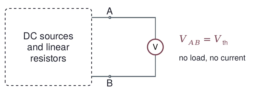
Vth is the open-circuit voltage

A dashed box labeled DC sources and linear resistors, with terminals A and B. A voltmeter is connected across A and B and nothing else. Beside it: V_AB equals V_th; no load, no current.

Vth=VOLV_{\text{th}} = V_{\text{OL}}: the voltage across A and B with the load removed.

A voltmeter draws almost no current, so it reads VthV_{\text{th}} directly.

© Ran Yang, Ph.D.Electronics
PHYS 252 · Lecture 0205

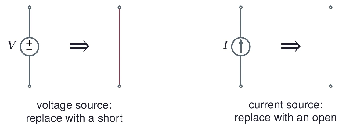
Zero the sources, then look in

Two rules side by side. Left: a voltage source V between two terminals, then an arrow, then a plain wire: replace a voltage source with a short. Right: a current source I between two terminals, then an arrow, then two unconnected terminals: replace a current source with an open.

Rth=ROLR_{\text{th}} = R_{\text{OL}}: the resistance between A and B with every source zeroed.

© Ran Yang, Ph.D.Electronics
PHYS 252 · Lecture 0206

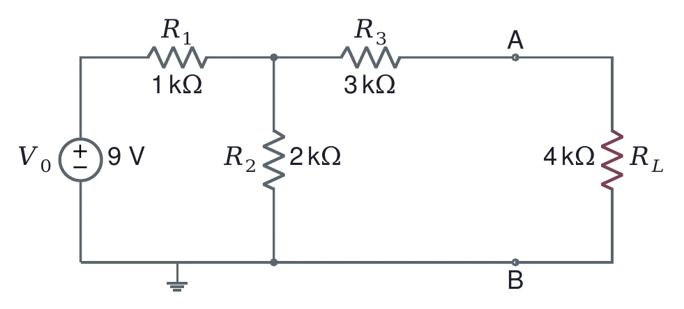
An example: 9 V and four resistors

The worked example circuit. A 9 V source V_0 feeds R_1 of 1 kilohm in series. From the node after R_1, R_2 of 2 kilohms goes to ground, and R_3 of 3 kilohms leads to terminal A. A load R_L of 4 kilohms connects terminal A to terminal B on the ground wire.

Find RthR_{\text{th}}, VthV_{\text{th}} and the load current ILI_L for RLR_L = 4 kΩ.

© Ran Yang, Ph.D.Electronics
PHYS 252 · Lecture 0207

Rth: short the source, remove the load
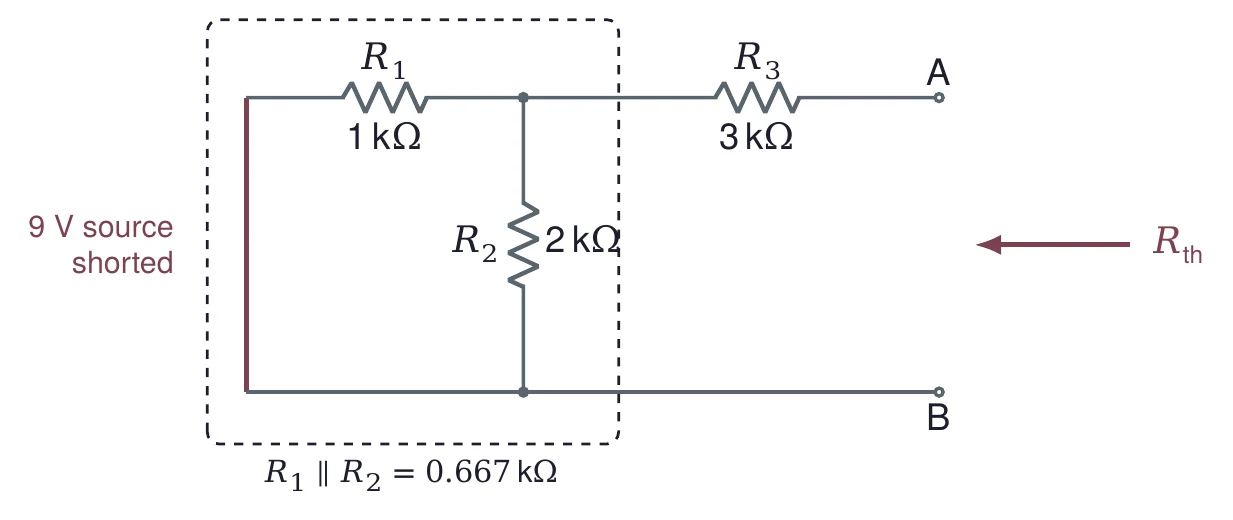
The worked example with the 9 V source replaced by a wire and the load removed. A dashed box around R_1 and R_2 notes that they are now in parallel: R_1 parallel R_2 = 0.667 kilohms. R_3 of 3 kilohms leads to terminal A. An arrow pointing into terminals A and B is labeled R_th.
Rth=R1∥R2+R3=1×21+2 kΩ+3 kΩ=113 kΩ=3.667 kΩR_{\text{th}} = R_1 \parallel R_2 + R_3 = \frac{1 \times 2}{1 + 2}\kohm + 3\kohm = \frac{11}{3}\kohm = 3.667\kohm
© Ran Yang, Ph.D.Electronics
PHYS 252 · Lecture 0208

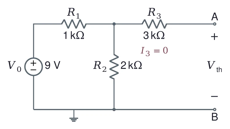
Vth: no load, no current in R3

The worked example with the load removed. The 9 V source drives R_1 of 1 kilohm and R_2 of 2 kilohms; R_3 of 3 kilohms leads to open terminal A and is marked I_3 = 0. The open-circuit voltage between A and B is labeled V_th, with plus at A.
I3=0  ⇒  Vth=VR2=9 V×21+2=6 VI_3 = 0 \;\Rightarrow\; V_{\text{th}} = V_{R_2} = 9\V \times \frac{2}{1 + 2} = 6\V
© Ran Yang, Ph.D.Electronics
PHYS 252 · Lecture 0209

Load the equivalent: 4 kΩ

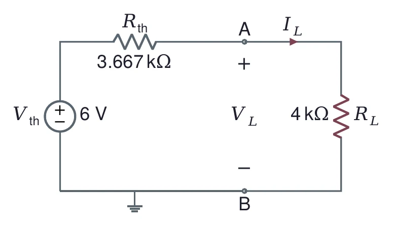
The Thévenin equivalent of the worked example: a 6 V source V_th in series with R_th of 3.667 kilohms, connected through terminals A and B to a 4 kilohm load R_L. The load current I_L flows from A into R_L, and the load voltage V_L is marked across A and B.
VL=6 V×43.667+4=3.130 VIL=3.130 V4 kΩ=0.783 mAV_L = 6\V \times \frac{4}{3.667 + 4} = 3.130\V \qquad I_L = \frac{3.130\V}{4\kohm} = 0.783\mA
© Ran Yang, Ph.D.Electronics
PHYS 252 · Lecture 0210

One equivalent, any load

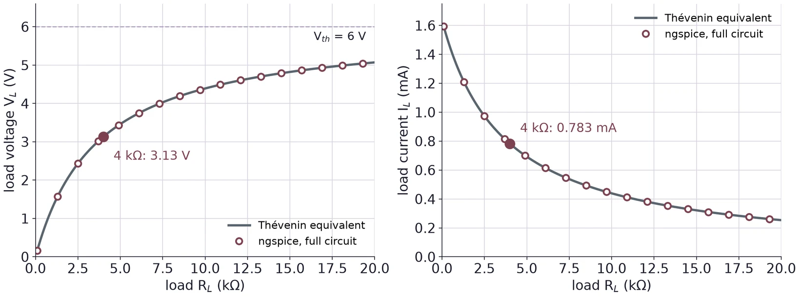
Two plots against load resistance from 0 to 20 kilohms for the worked example. Left: the load voltage V_L rises from near 0 toward the dashed V_th line at 6 V, passing 3.13 V at 4 kilohms. Right: the load current falls from about 1.6 mA, passing 0.783 mA at 4 kilohms. In both, open circles from an ngspice simulation of the full four-resistor circuit sit on the curve drawn from the Thévenin equivalent.

The circles are an ngspice simulation of the full four-resistor circuit. They land on the curves from the equivalent.

© Ran Yang, Ph.D.Electronics
PHYS 252 · Lecture 0211

Ladders: reduce one stage at a time

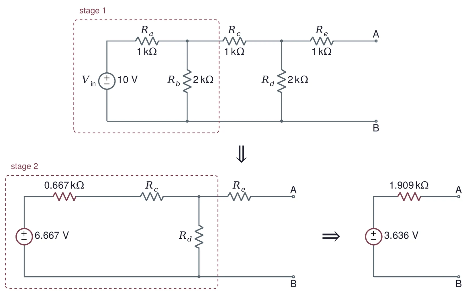
A two-stage ladder and its step-by-step reduction. Top: a 10 V source, series R_a of 1 kilohm, shunt R_b of 2 kilohms, series R_c of 1 kilohm, shunt R_d of 2 kilohms and series R_e of 1 kilohm to terminals A and B; the source, R_a and R_b are boxed as stage 1. Bottom left: stage 1 replaced by 6.667 V behind 0.667 kilohms, followed by R_c, R_d and R_e; the part up to R_d is boxed as stage 2. Bottom right: the whole ladder as 3.636 V behind 1.909 kilohms.

Stage 1: 10×2310 \times \tfrac{2}{3} = 6.667 V behind 1 kΩ ∥ 2 kΩ = 0.667 kΩ. Stage 2: 6.667×23.6676.667 \times \tfrac{2}{3.667} = 3.636 V behind 1.667 kΩ ∥ 2 kΩ = 0.909 kΩ, plus ReR_e.

© Ran Yang, Ph.D.Electronics
PHYS 252 · Lecture 0212

Part 2 · Impedance extends resistance

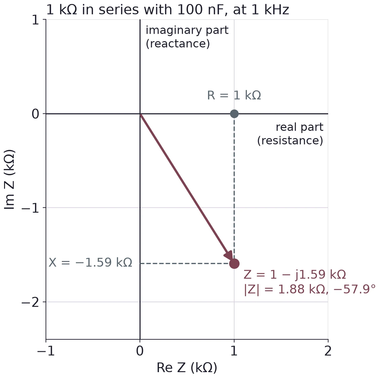
The complex impedance plane, real part (resistance) across and imaginary part (reactance) up, in kilohms. For 1 kilohm in series with 100 nF at 1 kHz, an arrow from the origin ends at Z = 1 minus j1.59 kilohms, with dashed lines to R = 1 kilohm on the real axis and X = minus 1.59 kilohms on the imaginary axis. The magnitude is 1.88 kilohms at minus 57.9 degrees.

Z=R+jXZ = R + jX, in ohms

PartImpedance
ResistorRR
Capacitor1jωC=−jωC\dfrac{1}{j\omega C} = -\dfrac{j}{\omega C}
InductorjωLj\omega L
© Ran Yang, Ph.D.Electronics
PHYS 252 · Lecture 0213

R and C together depend on time

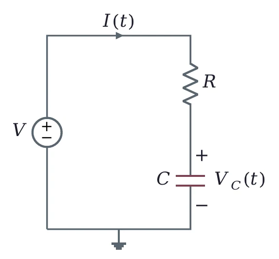
A source V drives a current I(t) through a resistor R and a capacitor C in series to ground. The capacitor voltage V_C(t) is marked across C.

With a capacitor, VV and II change with time.

Lecture 03 works this circuit.

For now: every source and every load has an impedance ZZ, and the divider rule holds for ZZ as it does for RR.

© Ran Yang, Ph.D.Electronics
PHYS 252 · Lecture 0214

Output impedance meets input impedance
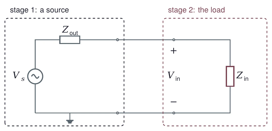
Two stages. Stage 1, a source, in a dashed box: an AC source V_s in series with an output impedance Z_out. Its output terminals connect to stage 2, the load, in a second dashed box: an input impedance Z_in, with the input voltage V_in marked across its terminals.
Vin=Vs ZinZout+ZinV_{\text{in}} = V_s\,\frac{Z_{\text{in}}}{Z_{\text{out}} + Z_{\text{in}}}
© Ran Yang, Ph.D.Electronics
PHYS 252 · Lecture 0215

You are the load

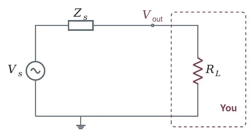
An AC source V_s in series with a source impedance Z_s drives a load resistor R_L. The voltage V_out is taken at the top of R_L. A dashed box around R_L is labeled You.
Vout=Vs RLZs+RLV_{\text{out}} = V_s\,\frac{R_L}{Z_s + R_L}

Whatever you connect, a meter, a scope or the next stage, takes its share of VsV_s.

© Ran Yang, Ph.D.Electronics
PHYS 252 · Lecture 0216

Bridging: make Zin at least ten times Zout
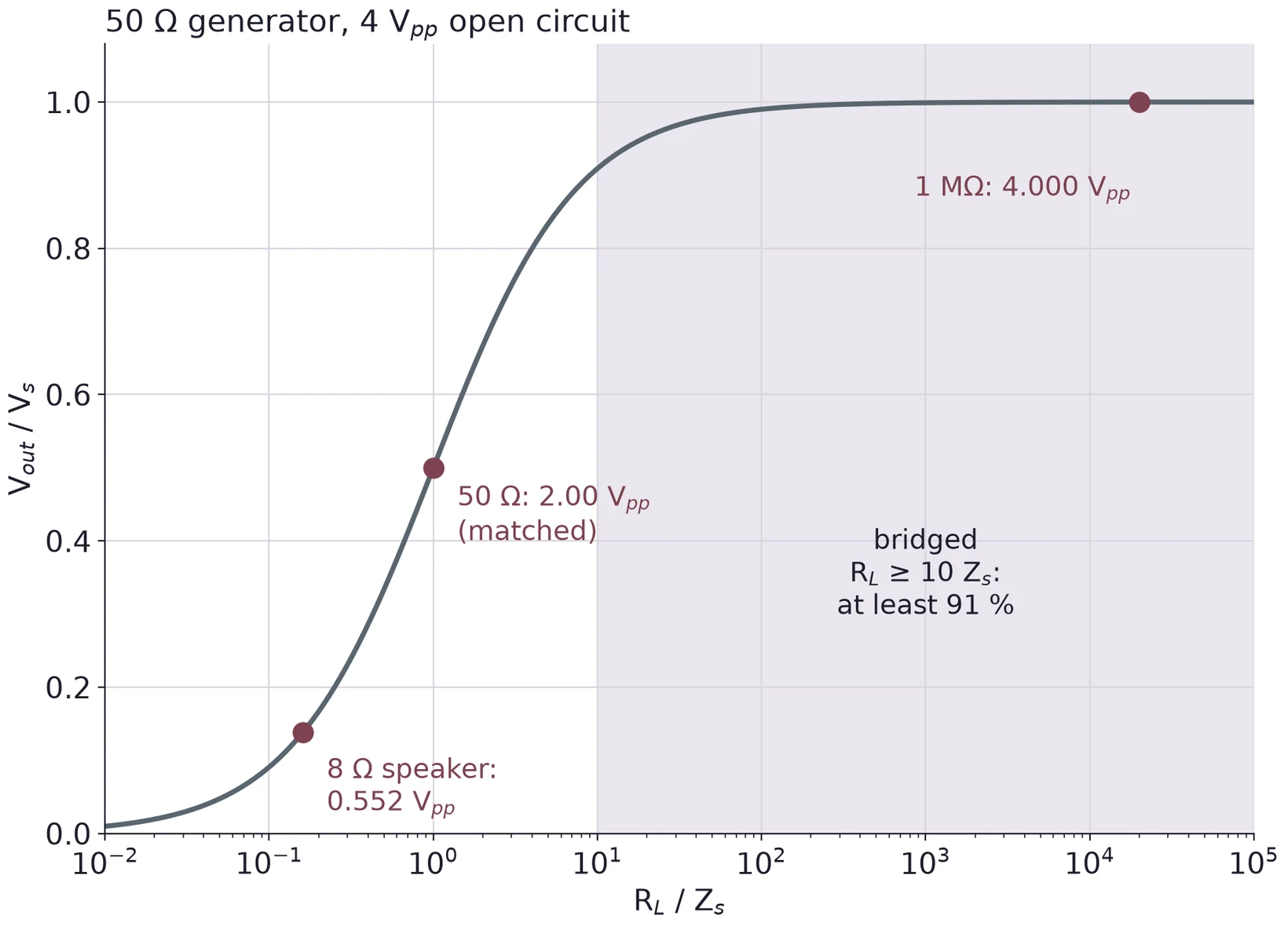
V_out over V_s against R_L over Z_s on a log axis from 0.01 to 100000, for a 50 ohm generator set to 4 V peak to peak open circuit. The S-shaped curve passes 0.138 for an 8 ohm speaker (0.552 V peak to peak), 0.5 for a matched 50 ohm load (2.00 V peak to peak) and nearly 1 for 1 megohm (4.000 V peak to peak). The region R_L at least 10 Z_s is shaded as bridged: at least 91 percent.
LoadVoutV_{\text{out}}
1 MΩ4.000 Vpp
50 Ω2.00 Vpp
8 Ω0.552 Vpp

A 50 Ω generator set for 4 Vpp open circuit. The 8 Ω speaker gets 4.76 mW.

© Ran Yang, Ph.D.Electronics
PHYS 252 · Lecture 0217

Part 3 · Power in the load: P = IV

The Thévenin equivalent of the worked example: a 6 V source V_th in series with R_th of 3.667 kilohms, connected through terminals A and B to a 4 kilohm load R_L. The load current I_L flows from A into R_L, and the load voltage V_L is marked across A and B.
PL=ILVL=VL2RL=0.783 mA×3.130 V=2.45 mWP_L = I_L V_L = \frac{V_L^2}{R_L} = 0.783\mA \times 3.130\V = 2.45\ \text{mW}

Is there a load that gets more?

© Ran Yang, Ph.D.Electronics
PHYS 252 · Lecture 0218

Power peaks at RL = Rth

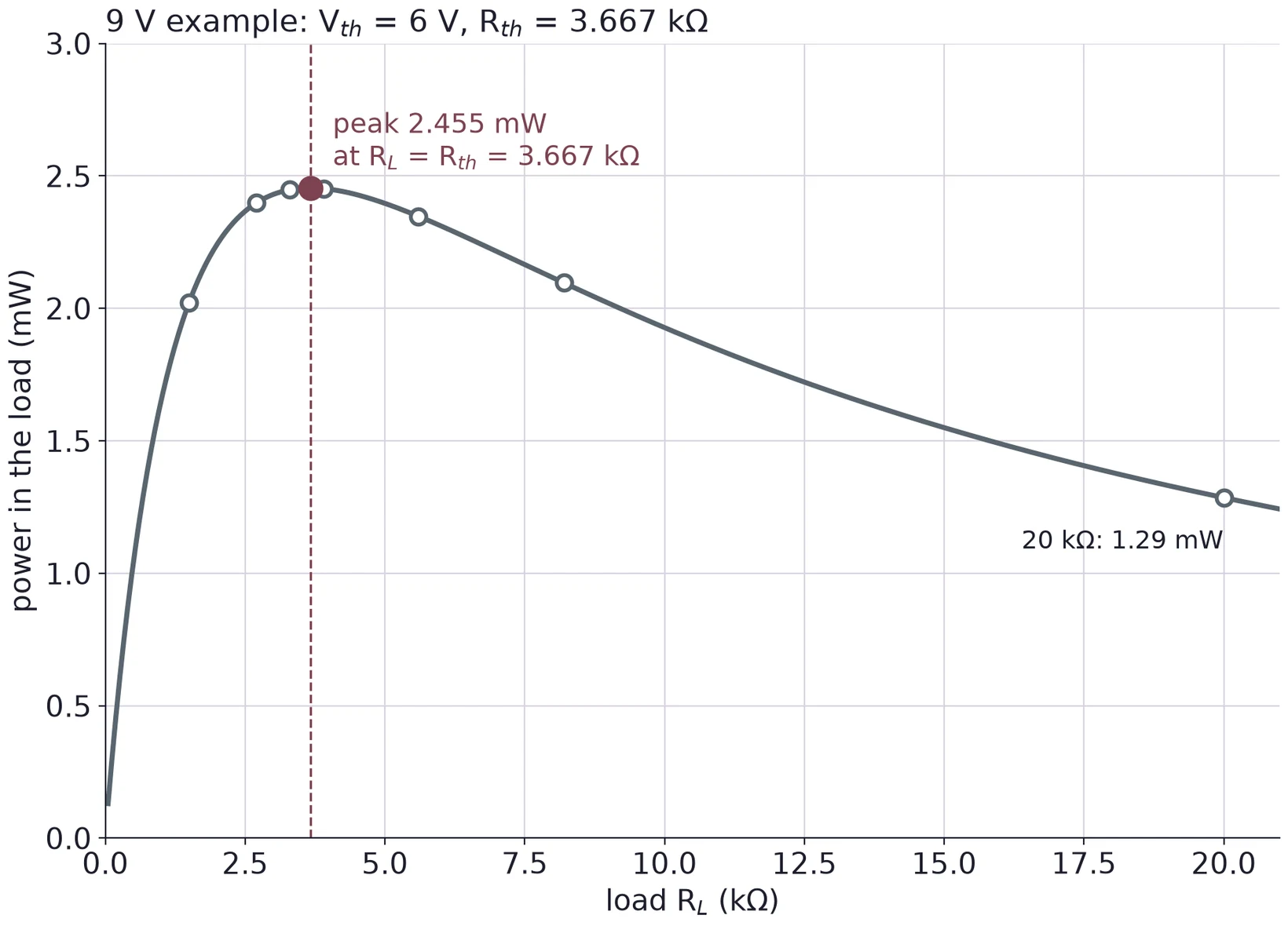
Power in the load against load resistance from 0 to 21 kilohms for the worked example, V_th = 6 V and R_th = 3.667 kilohms. The curve rises steeply, peaks at 2.455 mW where R_L equals R_th (dashed line), then falls slowly to 1.29 mW at 20 kilohms. Open circles mark 1.5, 2.7, 3.3, 3.9, 5.6, 8.2 and 20 kilohms.
P=Vth2RL(Rth+RL)2P = \frac{V_{\text{th}}^2 R_L}{(R_{\text{th}} + R_L)^2}dPdRL∝Rth−RL=0\frac{dP}{dR_L} \propto R_{\text{th}} - R_L = 0Pmax⁡=Vth24Rth=624×3.667 kΩP_{\max} = \frac{V_{\text{th}}^2}{4R_{\text{th}}} = \frac{6^2}{4 \times 3.667\kohm}=2.455 mW= 2.455\ \text{mW}
© Ran Yang, Ph.D.Electronics
PHYS 252 · Lecture 0219

Matched is not efficient

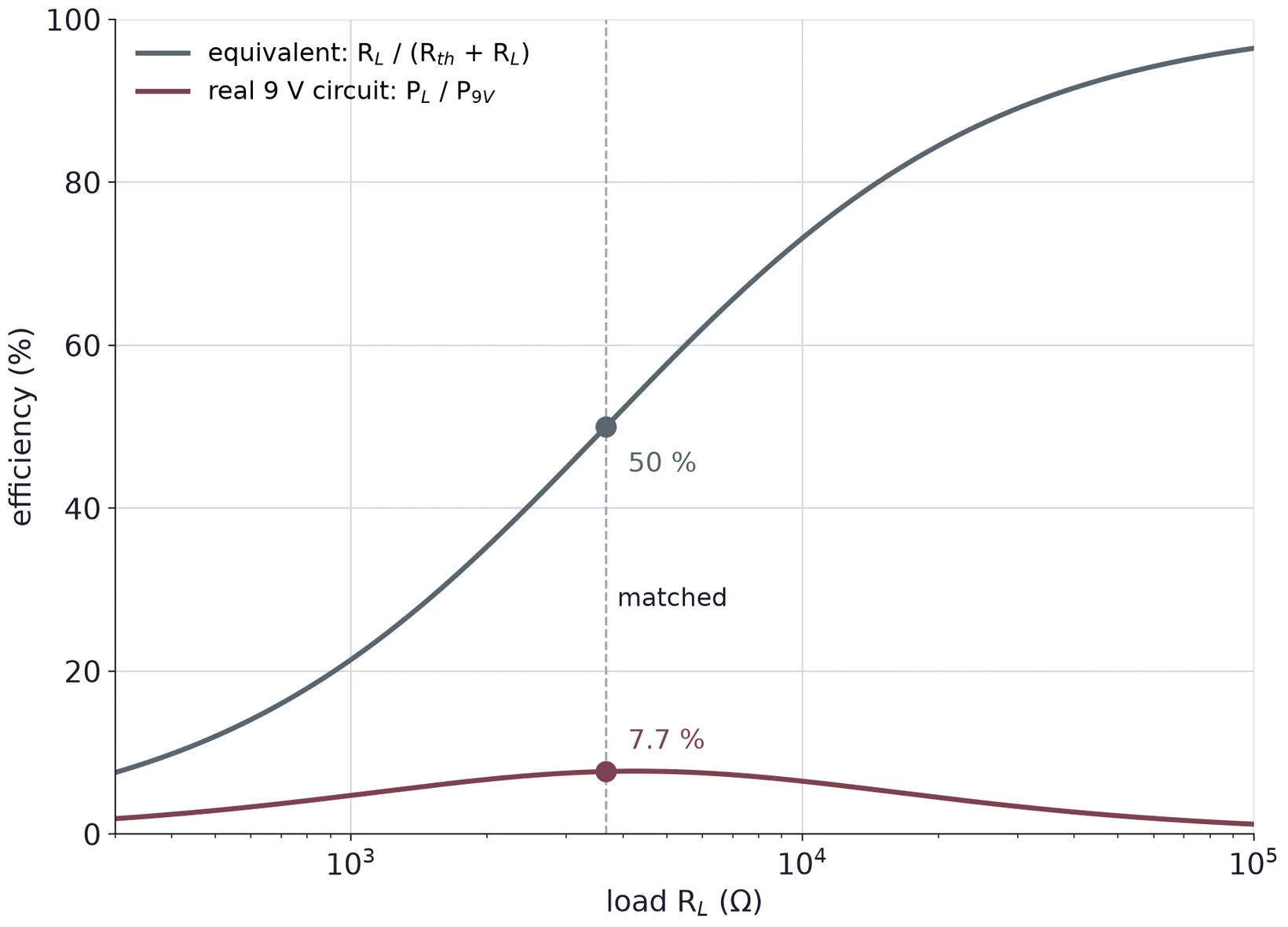
Efficiency in percent against load resistance from 300 ohms to 100 kilohms on a log axis. The Thévenin-equivalent efficiency R_L over (R_th + R_L) rises from about 8 to 96 percent and is 50 percent at the match, R_L = R_th = 3.667 kilohms (dashed line). The real 9 V circuit's efficiency, load power over the power the 9 V source supplies, stays below 8 percent and is 7.7 percent at the match.

At RLR_L = 3.667 kΩ:

Equiv.Real
Source4.91 mW31.91 mW
Load2.455 mW2.455 mW
Efficiency50 %7.7 %

The equivalent is right at the terminals only. Most of the real source's power heats R1R_1 and R2R_2.

© Ran Yang, Ph.D.Electronics
PHYS 252 · Lecture 0220

Match or bridge?

WhereChoice
RF, antennas, 50 Ω coaxMatched: most power, no reflections
Audio amplifier to speakerBridged: ZoutZ_{\text{out}} far below 8 Ω
Power gridBridged: efficiency first
Scope and DMM inputsBridged: read VocV_{\text{oc}}
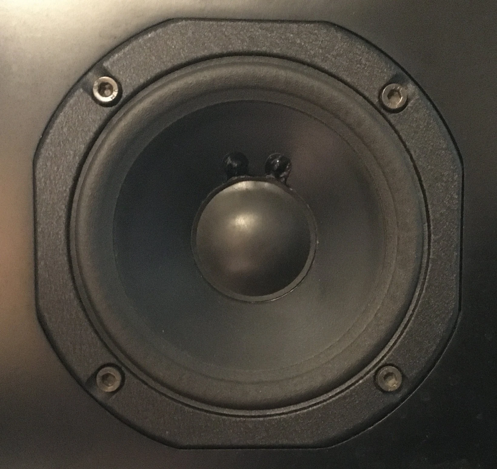
Front view of a round midrange loudspeaker driver with a dark cone and dust cap, mounted with four screws in a black cabinet.

Photo: Pittigrilli, CC BY-SA 4.0.

© Ran Yang, Ph.D.Electronics
PHYS 252 · Lecture 0221

The matched-load method

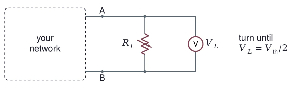
A dashed box labeled your network, with terminals A and B. A variable resistor R_L is connected across A and B, with a voltmeter reading V_L across it. Beside it: turn until V_L equals V_th over 2.

At VL=Vth/2V_L = V_{\text{th}}/2, the pot is at RthR_{\text{th}}.

For the 9 V example, stop at 3.00 V.

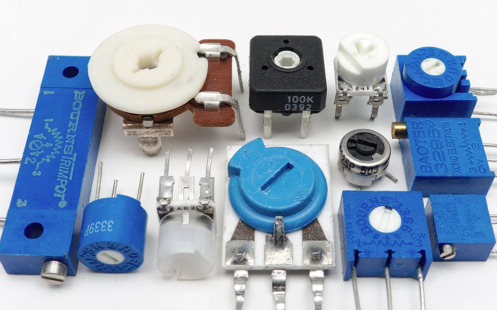
Twelve small board-mounted trimmer potentiometers of different shapes and sizes, single-turn and multi-turn, most in blue plastic.

Measure VthV_{\text{th}} first, with nothing connected. Photo: Junkyardsparkle, CC0.

© Ran Yang, Ph.D.Electronics
PHYS 252 · Lecture 0222

How exact is a match?

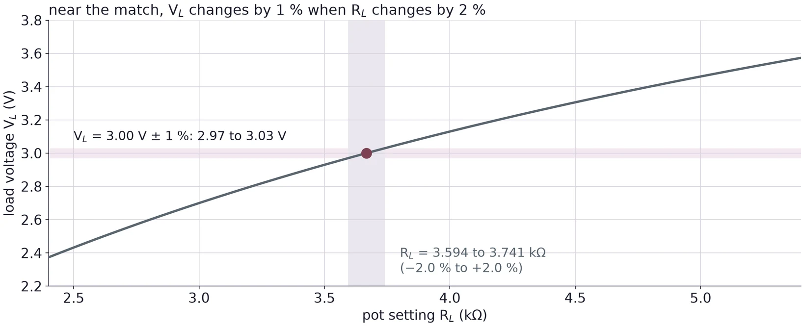
Load voltage against pot setting from 2.4 to 5.4 kilohms for the worked example. A horizontal band marks 3.00 V plus or minus 1 percent, 2.97 to 3.03 V. Where the curve crosses that band, a vertical band marks the pot settings that give it: 3.594 to 3.741 kilohms, minus 2.0 to plus 2.0 percent around R_th = 3.667 kilohms.
RLRth=1+ε1−ε≈1+2εε=1 %  ⇒  1.020\frac{R_L}{R_{\text{th}}} = \frac{1 + \varepsilon}{1 - \varepsilon} \approx 1 + 2\varepsilon \qquad \varepsilon = 1\,\% \;\Rightarrow\; 1.020
© Ran Yang, Ph.D.Electronics
PHYS 252 · Lecture 0223

The known-load method

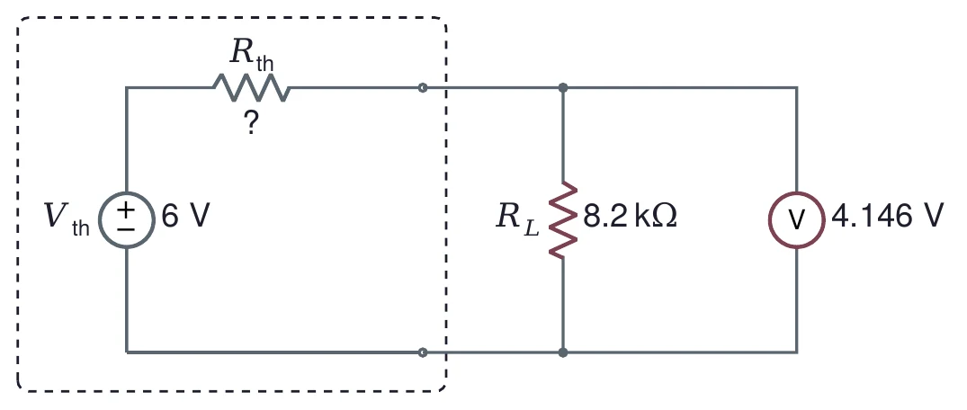
Inside a dashed box, a source V_th of 6 V in series with an unknown R_th marked with a question mark. A known load R_L of 8.2 kilohms is connected across the output, with a voltmeter reading 4.146 V.
Rth=RL(VthVL−1)=8.2 kΩ×(64.146−1)=3.667 kΩR_{\text{th}} = R_L\left(\frac{V_{\text{th}}}{V_L} - 1\right) = 8.2\kohm \times \left(\frac{6}{4.146} - 1\right) = 3.667\kohm

One fixed resistor and two voltage readings. No pot to turn.

© Ran Yang, Ph.D.Electronics
PHYS 252 · Lecture 0224

Part 4 · Kirchhoff's current law at a node
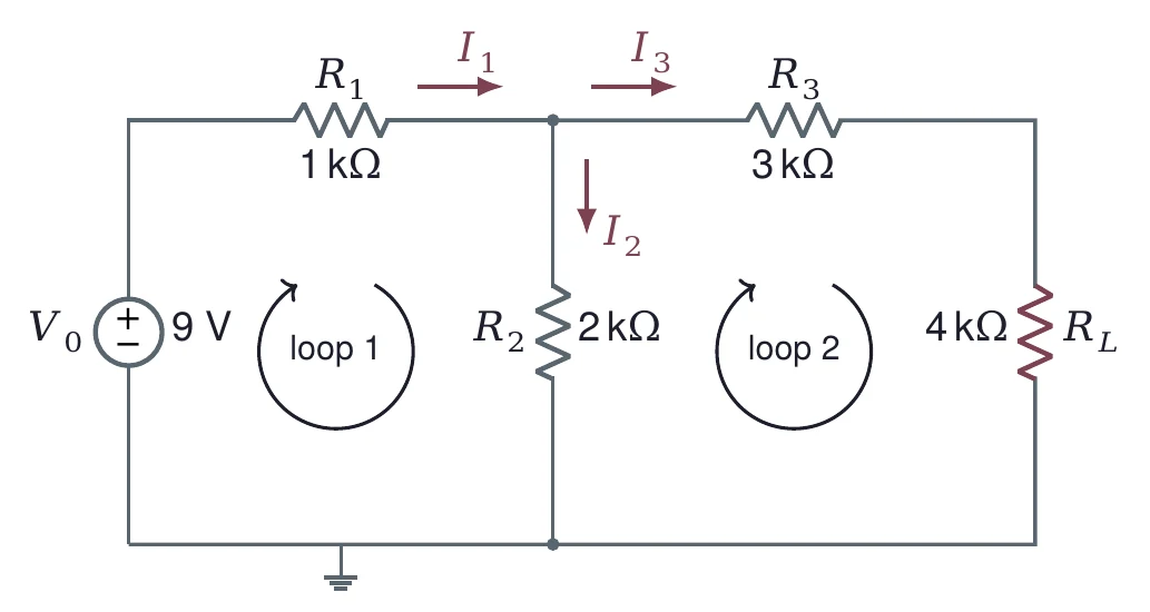
The worked example circuit with currents and loops. A 9 V source V_0, R_1 of 1 kilohm in series, R_2 of 2 kilohms as a shunt, then R_3 of 3 kilohms and R_L of 4 kilohms. Arrows mark I_1 into the top node through R_1, I_2 down through R_2 and I_3 out through R_3. Clockwise arrows mark loop 1 through the source, R_1 and R_2, and loop 2 through R_2, R_3 and R_L.
I1=I2+I39 V=R1I1+R2I20=−R2I2+(R3+RL)I3I_1 = I_2 + I_3 \qquad 9\V = R_1 I_1 + R_2 I_2 \qquad 0 = -R_2 I_2 + (R_3 + R_L) I_3

Current in = current out at the top node. Around each loop, the voltages add to zero.

© Ran Yang, Ph.D.Electronics
PHYS 252 · Lecture 0225

Three equations, three unknowns

[1−1−1R1R200−R2R3+RL][I1I2I3]=[09 V0]\begin{bmatrix} 1 & -1 & -1 \\ R_1 & R_2 & 0 \\ 0 & -R_2 & R_3 + R_L \end{bmatrix} \begin{bmatrix} I_1 \\ I_2 \\ I_3 \end{bmatrix} = \begin{bmatrix} 0 \\ 9\V \\ 0 \end{bmatrix}
The worked example circuit with currents and loops. A 9 V source V_0, R_1 of 1 kilohm in series, R_2 of 2 kilohms as a shunt, then R_3 of 3 kilohms and R_L of 4 kilohms. Arrows mark I_1 into the top node through R_1, I_2 down through R_2 and I_3 out through R_3. Clockwise arrows mark loop 1 through the source, R_1 and R_2, and loop 2 through R_2, R_3 and R_L.

R I=V\mathbf{R}\,\mathbf{I} = \mathbf{V}. Row 1 is the current law at the top node; rows 2 and 3 are loops 1 and 2, with R1R_1 = 1 kΩ, R2R_2 = 2 kΩ, R3+RLR_3 + R_L = 7 kΩ.

© Ran Yang, Ph.D.Electronics
PHYS 252 · Lecture 0226

numpy.linalg.solve does the algebra

import numpy as np
R = np.array([[1,    -1,   -1],
              [1e3,  2e3,  0],
              [0,   -2e3,  7e3]])
V = np.array([0, 9, 0])
I = np.linalg.solve(R, V)
print(I * 1e3)          # in mA

Example only. Do not copy this code as it is: read it, learn from it, then write your own.

[3.52173913 2.73913043 0.7826087 ]

I3I_3 = 0.783 mA, the same as the Thévenin answer. Two loop currents give a 2 × 2 system with the same I3I_3.

© Ran Yang, Ph.D.Example code only: learn from it, then write your ownElectronics
PHYS 252 · Lecture 0227

Part 5 · A source's resistance from many loads
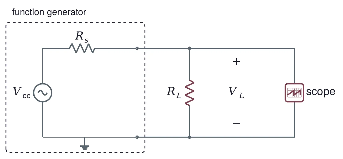
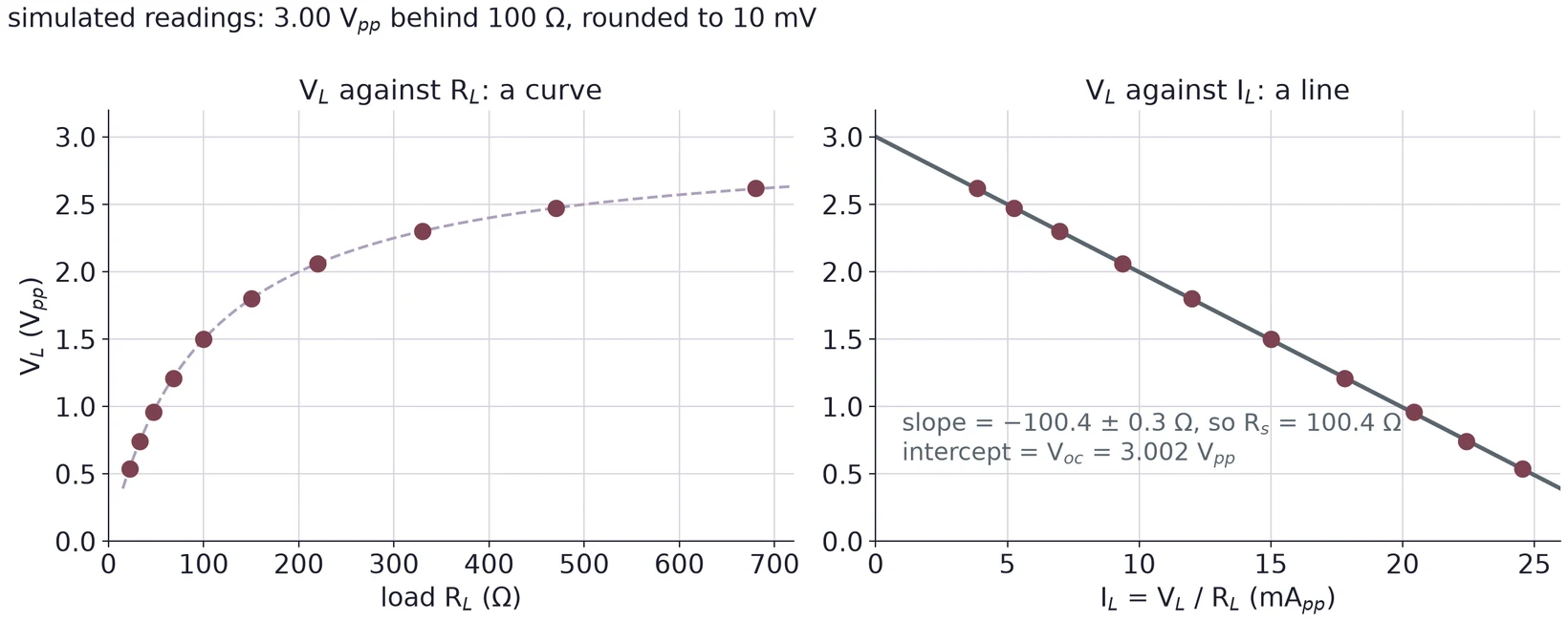
A function generator in a dashed box, modeled as an AC source V_oc in series with R_s. Its output drives a load resistor R_L, and a scope is connected across the load. The load voltage V_L is marked between them.
VL=Voc RLRs+RLV_L = V_{\text{oc}}\,\frac{R_L}{R_s + R_L}
© Ran Yang, Ph.D.Electronics
PHYS 252 · Lecture 0228

Make it a straight line

Two plots of the same simulated readings from a 3.00 V peak-to-peak source behind 100 ohms, rounded to 10 mV. Left: V_L against R_L from 22 to 680 ohms, a curve rising from 0.54 to 2.62 V. Right: V_L against I_L = V_L over R_L, the points fall on a straight line; the fit has slope minus 100.4 plus or minus 0.3 ohms, so R_s = 100.4 ohms, and intercept V_oc = 3.002 V peak to peak.

VL=Voc−RsILV_L = V_{\text{oc}} - R_s I_L, so a line through (ILI_L, VLV_L) has slope −Rs-R_s. Simulated readings: RsR_s = 100.4 ± 0.3 Ω, VocV_{\text{oc}} = 3.002 Vpp.

© Ran Yang, Ph.D.Electronics
PHYS 252 · Lecture 0229

Which loads tell you the most?

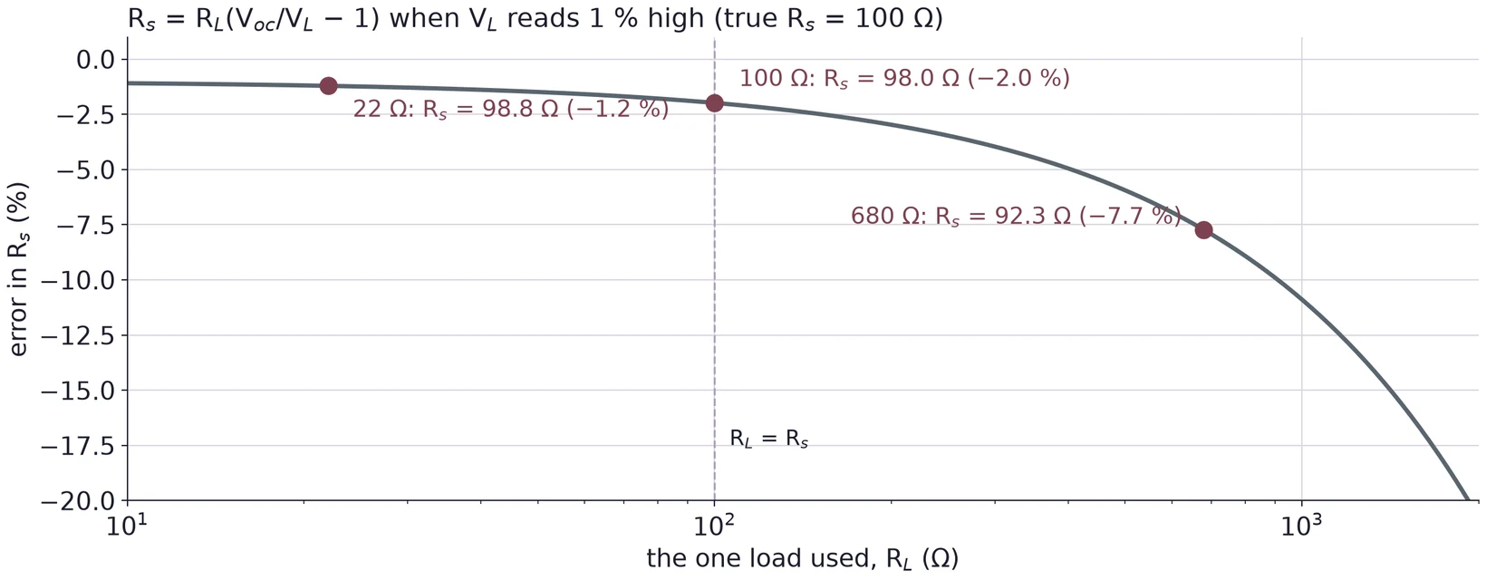
Percent error in R_s, computed from a single load as R_L(V_oc over V_L minus 1), when V_L reads 1 percent high and the true R_s is 100 ohms, against the load on a log axis from 10 to 2000 ohms. The error is minus 1.2 percent at 22 ohms (98.8 ohms), minus 2.0 percent at 100 ohms (98.0 ohms), minus 7.7 percent at 680 ohms (92.3 ohms) and grows quickly above that. A dashed line marks R_L = R_s.

A load far above RsR_s barely pulls VLV_L down, so a small reading error looks like a big change in RsR_s. Use loads near RsR_s and below it.

© Ran Yang, Ph.D.Electronics
PHYS 252 · Lecture 0230

Part 6 · Offset moves the wave, not its shape
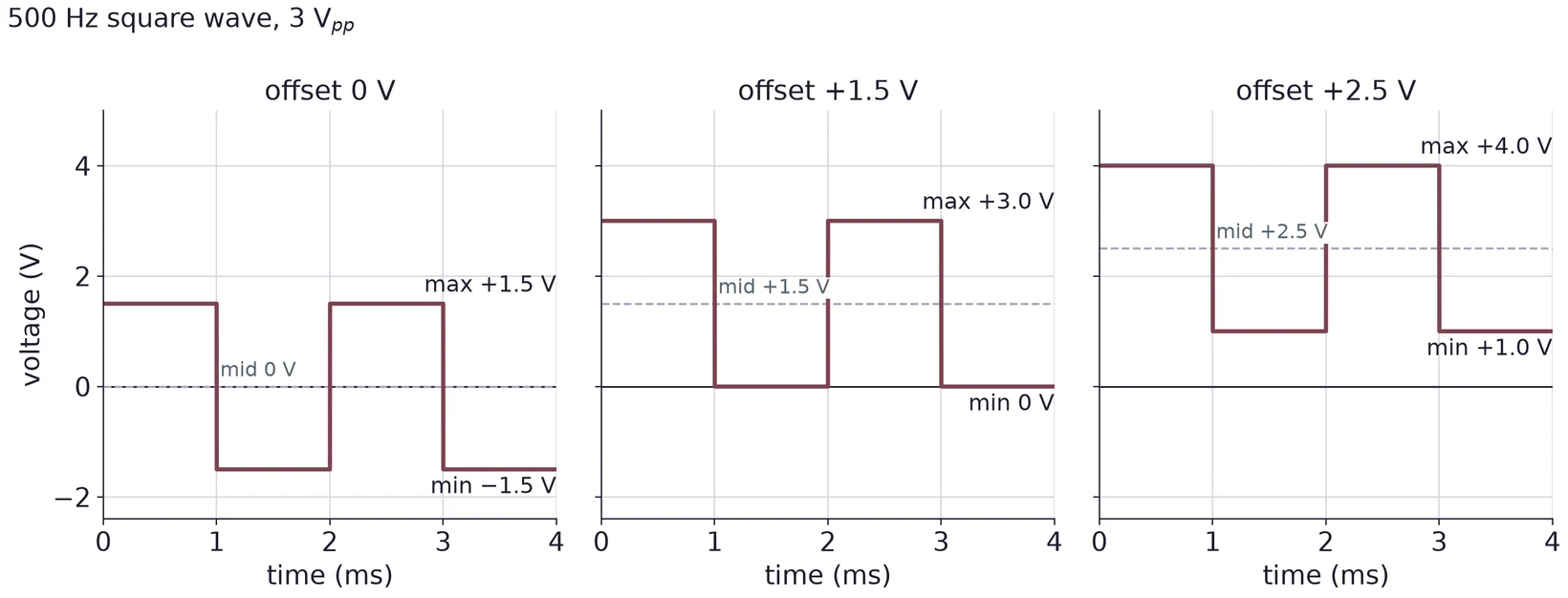
Three panels of a 500 Hz, 3 V peak-to-peak square wave against time from 0 to 4 ms. Offset 0 V: from minus 1.5 to plus 1.5 V, middle 0 V. Offset plus 1.5 V: from 0 to plus 3.0 V, middle plus 1.5 V. Offset plus 2.5 V: from plus 1.0 to plus 4.0 V, middle plus 2.5 V. The shape is the same in all three; only the middle moves.
Vmax⁡=Voffset+12VppVmin⁡=Voffset−12VppV_{\max} = V_{\text{offset}} + \tfrac{1}{2}V_{pp} \qquad V_{\min} = V_{\text{offset}} - \tfrac{1}{2}V_{pp}
© Ran Yang, Ph.D.Electronics
PHYS 252 · Lecture 0231

Put the trigger level between min and max
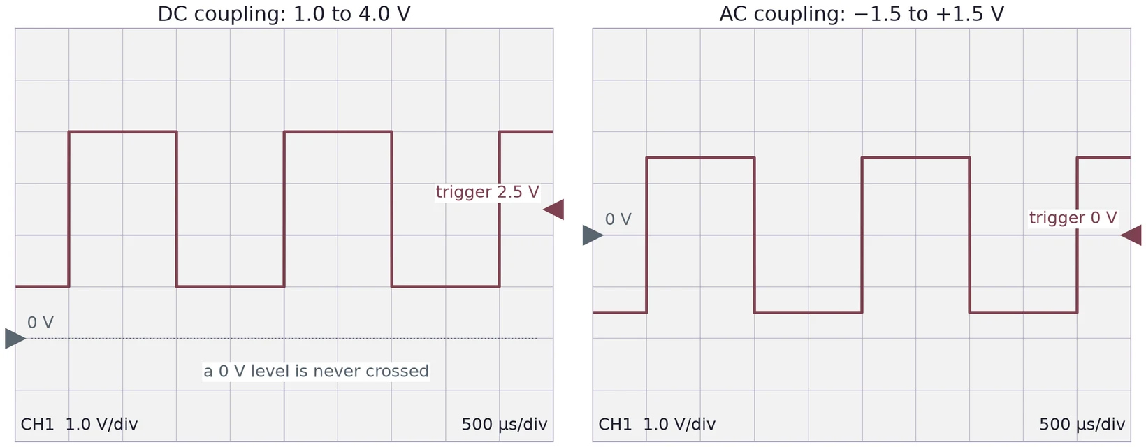
Two scope screens at 1 V per division and 500 microseconds per division. Left, DC coupling: the plus 2.5 V offset square wave runs from 1.0 to 4.0 V above a ground marker two divisions below center; the trigger marker sits at 2.5 V, and a dotted 0 V line is labeled a 0 V level is never crossed. Right, AC coupling: the same wave centered on 0 V, from minus 1.5 to plus 1.5 V, with the trigger at 0 V.

DC coupling shows the offset, so the level must move with it. AC coupling removes the average, and 0 V works again.

© Ran Yang, Ph.D.Electronics
PHYS 252 · Lecture 0232

Cursors for max, min and peak-to-peak

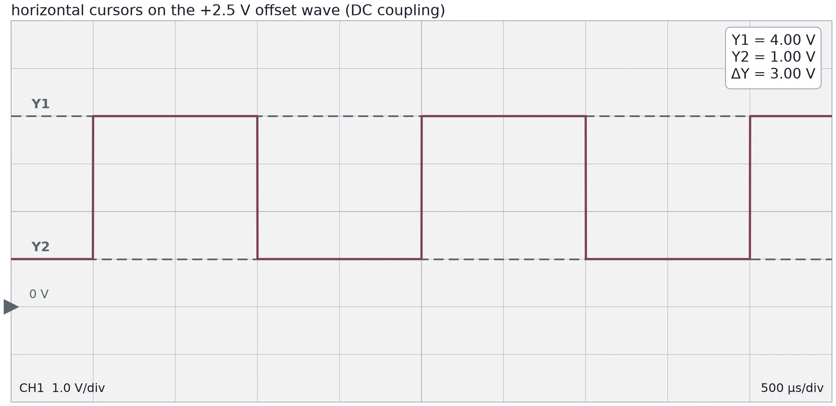
A scope screen at 1 V per division and 500 microseconds per division showing the plus 2.5 V offset square wave in DC coupling, ground marker two divisions below center. Horizontal cursor Y1 lies on the top of the wave and Y2 on the bottom. A readout box shows Y1 = 4.00 V, Y2 = 1.00 V, delta Y = 3.00 V.

Set Y1 on the top of the wave and Y2 on the bottom. Read max, min and ΔY = VppV_{pp} in DC coupling.

© Ran Yang, Ph.D.Electronics
PHYS 252 · Lecture 0233

Error analysis in every task

ResultMain error sources
VthV_{\text{th}} and node voltagesResistor tolerance, supply setting, DMM accuracy
RthR_{\text{th}}, matched loadReading Vth/2V_{\text{th}}/2 (×2 in RR), measuring the pot afterwards
Power against RLR_LErrors in VLV_L count twice in VL2/RLV_L^2/R_L
RsR_s by regressionSlope uncertainty, scope reading, choice of loads
Max, min, VppV_{pp}Cursor placement, trace thickness, coupling

For each value: state the uncertainty, name the main sources, and compare with what you expected.

© Ran Yang, Ph.D.Electronics

Use ← → to move, Home / End to jump, and F for fullscreen.

Figure descriptions

Slide 2 · Part 1 · Lab 2 in five tasks

Lab 2 in four rows. Network analysis: Task 1, build the network and find V_th and the node voltages. Impedance matching: Task 2, the matched-load method with a pot to find R_th, then Task 3, four loads and a plot of power against load resistance. Function generator: Task 4, ten loads and a regression to find R_s. Triggering: Task 5, offset square waves, trigger level and cursors.

Slide 3 · Any linear circuit looks like one source and one resistor

Left: a dashed box labeled DC sources and linear resistors, with terminals A and B connected to a load resistor R_L. An arrow points right to the equivalent: inside a dashed box, a source V_th in series with a resistor R_th, connected through terminals A and B to the same load R_L.

Slide 4 · Vth is the open-circuit voltage

A dashed box labeled DC sources and linear resistors, with terminals A and B. A voltmeter is connected across A and B and nothing else. Beside it: V_AB equals V_th; no load, no current.

Slide 5 · Zero the sources, then look in

Two rules side by side. Left: a voltage source V between two terminals, then an arrow, then a plain wire: replace a voltage source with a short. Right: a current source I between two terminals, then an arrow, then two unconnected terminals: replace a current source with an open.

Slide 6 · An example: 9 V and four resistors

The worked example circuit. A 9 V source V_0 feeds R_1 of 1 kilohm in series. From the node after R_1, R_2 of 2 kilohms goes to ground, and R_3 of 3 kilohms leads to terminal A. A load R_L of 4 kilohms connects terminal A to terminal B on the ground wire.

Slide 7 · Rth: short the source, remove the load

The worked example with the 9 V source replaced by a wire and the load removed. A dashed box around R_1 and R_2 notes that they are now in parallel: R_1 parallel R_2 = 0.667 kilohms. R_3 of 3 kilohms leads to terminal A. An arrow pointing into terminals A and B is labeled R_th.

Slide 8 · Vth: no load, no current in R3

The worked example with the load removed. The 9 V source drives R_1 of 1 kilohm and R_2 of 2 kilohms; R_3 of 3 kilohms leads to open terminal A and is marked I_3 = 0. The open-circuit voltage between A and B is labeled V_th, with plus at A.

Slide 9 · Load the equivalent: 4 kΩ

The Thévenin equivalent of the worked example: a 6 V source V_th in series with R_th of 3.667 kilohms, connected through terminals A and B to a 4 kilohm load R_L. The load current I_L flows from A into R_L, and the load voltage V_L is marked across A and B.

Slide 10 · One equivalent, any load

Two plots against load resistance from 0 to 20 kilohms for the worked example. Left: the load voltage V_L rises from near 0 toward the dashed V_th line at 6 V, passing 3.13 V at 4 kilohms. Right: the load current falls from about 1.6 mA, passing 0.783 mA at 4 kilohms. In both, open circles from an ngspice simulation of the full four-resistor circuit sit on the curve drawn from the Thévenin equivalent.

Slide 11 · Ladders: reduce one stage at a time

A two-stage ladder and its step-by-step reduction. Top: a 10 V source, series R_a of 1 kilohm, shunt R_b of 2 kilohms, series R_c of 1 kilohm, shunt R_d of 2 kilohms and series R_e of 1 kilohm to terminals A and B; the source, R_a and R_b are boxed as stage 1. Bottom left: stage 1 replaced by 6.667 V behind 0.667 kilohms, followed by R_c, R_d and R_e; the part up to R_d is boxed as stage 2. Bottom right: the whole ladder as 3.636 V behind 1.909 kilohms.

Slide 12 · Part 2 · Impedance extends resistance

The complex impedance plane, real part (resistance) across and imaginary part (reactance) up, in kilohms. For 1 kilohm in series with 100 nF at 1 kHz, an arrow from the origin ends at Z = 1 minus j1.59 kilohms, with dashed lines to R = 1 kilohm on the real axis and X = minus 1.59 kilohms on the imaginary axis. The magnitude is 1.88 kilohms at minus 57.9 degrees.

Slide 13 · R and C together depend on time

A source V drives a current I(t) through a resistor R and a capacitor C in series to ground. The capacitor voltage V_C(t) is marked across C.

Slide 14 · Output impedance meets input impedance

Two stages. Stage 1, a source, in a dashed box: an AC source V_s in series with an output impedance Z_out. Its output terminals connect to stage 2, the load, in a second dashed box: an input impedance Z_in, with the input voltage V_in marked across its terminals.

Slide 15 · You are the load

An AC source V_s in series with a source impedance Z_s drives a load resistor R_L. The voltage V_out is taken at the top of R_L. A dashed box around R_L is labeled You.

Slide 16 · Bridging: make Zin at least ten times Zout

V_out over V_s against R_L over Z_s on a log axis from 0.01 to 100000, for a 50 ohm generator set to 4 V peak to peak open circuit. The S-shaped curve passes 0.138 for an 8 ohm speaker (0.552 V peak to peak), 0.5 for a matched 50 ohm load (2.00 V peak to peak) and nearly 1 for 1 megohm (4.000 V peak to peak). The region R_L at least 10 Z_s is shaded as bridged: at least 91 percent.

Slide 17 · Part 3 · Power in the load: P = IV

The Thévenin equivalent of the worked example: a 6 V source V_th in series with R_th of 3.667 kilohms, connected through terminals A and B to a 4 kilohm load R_L. The load current I_L flows from A into R_L, and the load voltage V_L is marked across A and B.

Slide 18 · Power peaks at RL = Rth

Power in the load against load resistance from 0 to 21 kilohms for the worked example, V_th = 6 V and R_th = 3.667 kilohms. The curve rises steeply, peaks at 2.455 mW where R_L equals R_th (dashed line), then falls slowly to 1.29 mW at 20 kilohms. Open circles mark 1.5, 2.7, 3.3, 3.9, 5.6, 8.2 and 20 kilohms.

Slide 19 · Matched is not efficient

Efficiency in percent against load resistance from 300 ohms to 100 kilohms on a log axis. The Thévenin-equivalent efficiency R_L over (R_th + R_L) rises from about 8 to 96 percent and is 50 percent at the match, R_L = R_th = 3.667 kilohms (dashed line). The real 9 V circuit's efficiency, load power over the power the 9 V source supplies, stays below 8 percent and is 7.7 percent at the match.

Slide 20 · Match or bridge?

Front view of a round midrange loudspeaker driver with a dark cone and dust cap, mounted with four screws in a black cabinet.

Slide 21 · The matched-load method

A dashed box labeled your network, with terminals A and B. A variable resistor R_L is connected across A and B, with a voltmeter reading V_L across it. Beside it: turn until V_L equals V_th over 2.

Twelve small board-mounted trimmer potentiometers of different shapes and sizes, single-turn and multi-turn, most in blue plastic.

Slide 22 · How exact is a match?

Load voltage against pot setting from 2.4 to 5.4 kilohms for the worked example. A horizontal band marks 3.00 V plus or minus 1 percent, 2.97 to 3.03 V. Where the curve crosses that band, a vertical band marks the pot settings that give it: 3.594 to 3.741 kilohms, minus 2.0 to plus 2.0 percent around R_th = 3.667 kilohms.

Slide 23 · The known-load method

Inside a dashed box, a source V_th of 6 V in series with an unknown R_th marked with a question mark. A known load R_L of 8.2 kilohms is connected across the output, with a voltmeter reading 4.146 V.

Slide 24 · Part 4 · Kirchhoff's current law at a node

The worked example circuit with currents and loops. A 9 V source V_0, R_1 of 1 kilohm in series, R_2 of 2 kilohms as a shunt, then R_3 of 3 kilohms and R_L of 4 kilohms. Arrows mark I_1 into the top node through R_1, I_2 down through R_2 and I_3 out through R_3. Clockwise arrows mark loop 1 through the source, R_1 and R_2, and loop 2 through R_2, R_3 and R_L.

Slide 25 · Three equations, three unknowns

The worked example circuit with currents and loops. A 9 V source V_0, R_1 of 1 kilohm in series, R_2 of 2 kilohms as a shunt, then R_3 of 3 kilohms and R_L of 4 kilohms. Arrows mark I_1 into the top node through R_1, I_2 down through R_2 and I_3 out through R_3. Clockwise arrows mark loop 1 through the source, R_1 and R_2, and loop 2 through R_2, R_3 and R_L.

Slide 27 · Part 5 · A source's resistance from many loads

A function generator in a dashed box, modeled as an AC source V_oc in series with R_s. Its output drives a load resistor R_L, and a scope is connected across the load. The load voltage V_L is marked between them.

Slide 28 · Make it a straight line

Two plots of the same simulated readings from a 3.00 V peak-to-peak source behind 100 ohms, rounded to 10 mV. Left: V_L against R_L from 22 to 680 ohms, a curve rising from 0.54 to 2.62 V. Right: V_L against I_L = V_L over R_L, the points fall on a straight line; the fit has slope minus 100.4 plus or minus 0.3 ohms, so R_s = 100.4 ohms, and intercept V_oc = 3.002 V peak to peak.

Slide 29 · Which loads tell you the most?

Percent error in R_s, computed from a single load as R_L(V_oc over V_L minus 1), when V_L reads 1 percent high and the true R_s is 100 ohms, against the load on a log axis from 10 to 2000 ohms. The error is minus 1.2 percent at 22 ohms (98.8 ohms), minus 2.0 percent at 100 ohms (98.0 ohms), minus 7.7 percent at 680 ohms (92.3 ohms) and grows quickly above that. A dashed line marks R_L = R_s.

Slide 30 · Part 6 · Offset moves the wave, not its shape

Three panels of a 500 Hz, 3 V peak-to-peak square wave against time from 0 to 4 ms. Offset 0 V: from minus 1.5 to plus 1.5 V, middle 0 V. Offset plus 1.5 V: from 0 to plus 3.0 V, middle plus 1.5 V. Offset plus 2.5 V: from plus 1.0 to plus 4.0 V, middle plus 2.5 V. The shape is the same in all three; only the middle moves.

Slide 31 · Put the trigger level between min and max

Two scope screens at 1 V per division and 500 microseconds per division. Left, DC coupling: the plus 2.5 V offset square wave runs from 1.0 to 4.0 V above a ground marker two divisions below center; the trigger marker sits at 2.5 V, and a dotted 0 V line is labeled a 0 V level is never crossed. Right, AC coupling: the same wave centered on 0 V, from minus 1.5 to plus 1.5 V, with the trigger at 0 V.

Slide 32 · Cursors for max, min and peak-to-peak

A scope screen at 1 V per division and 500 microseconds per division showing the plus 2.5 V offset square wave in DC coupling, ground marker two divisions below center. Horizontal cursor Y1 lies on the top of the wave and Y2 on the bottom. A readout box shows Y1 = 4.00 V, Y2 = 1.00 V, delta Y = 3.00 V.