Part 1 · Lab 3 in five tasks
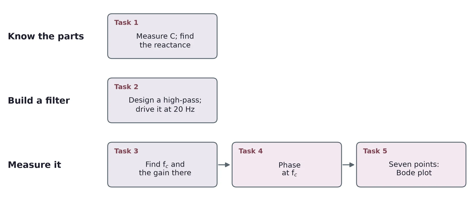
First you measure capacitors. Then you build one filter and measure how it treats each frequency: its cutoff, its phase and its Bode plot.
A capacitor stores charge
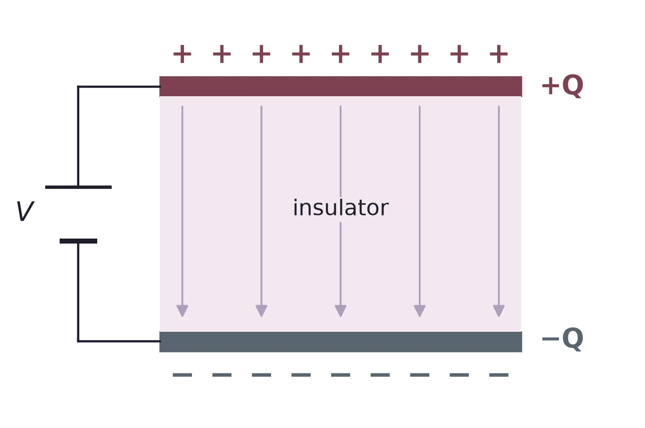
in farads: 1 F = 1 C/V.
47 µF at 9 V:
Real parts run from picofarads (pF) to thousands of microfarads (µF).
Polarized and non-polarized
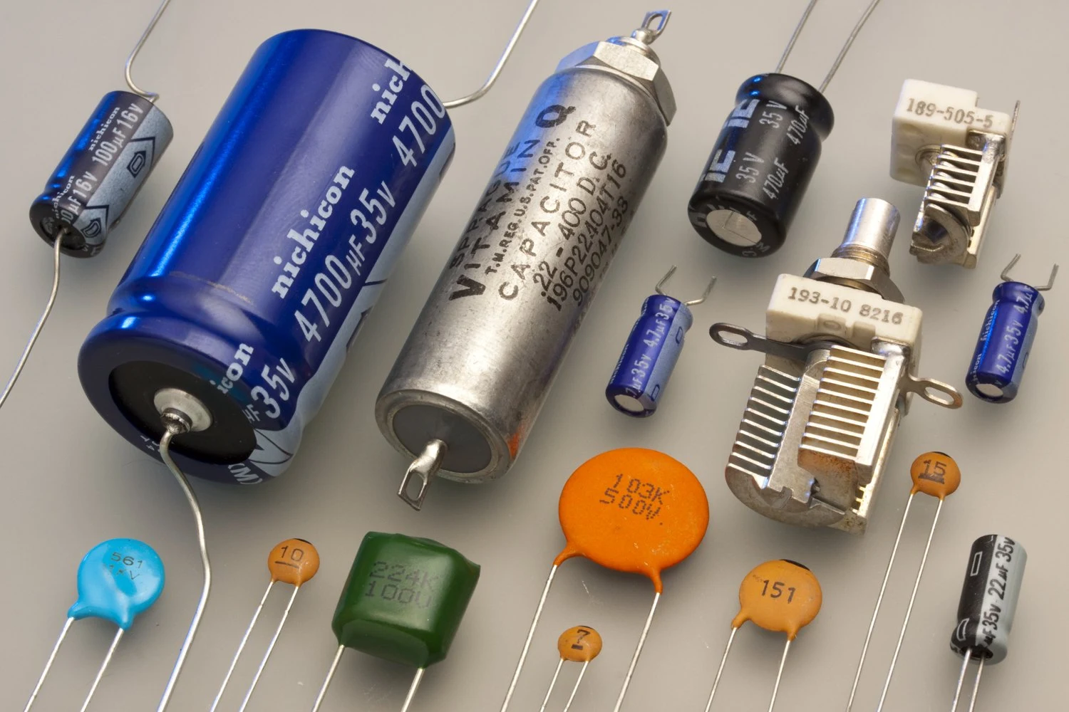
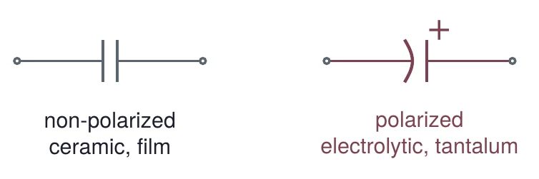
An electrolytic has a + lead. Connect it to the higher voltage.
Blue and black cans: electrolytic. Orange and blue discs: ceramic. Green block: film. Photo: Eric Schrader, CC BY-SA 2.0.

Three kinds side by side
| Kind | Range | Tolerance | Polarized? |
|---|---|---|---|
| Aluminum electrolytic | 1 to 22 000 µF | ±20 % | yes |
| Ceramic (C0G, X7R) | 10 pF to 1 µF | ±5, 10 or 20 % | no |
| Film (polyester) | 0.01 to 4.7 µF | ±5, 10 or 20 % | no |
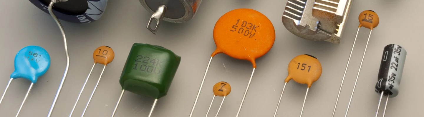
Ranges from one series each: Nichicon UVR, Vishay K series, WIMA MKS 2. Photo: Eric Schrader, CC BY-SA 2.0.
The electrolytic datasheet
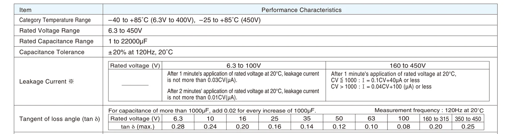
Capacitance tolerance: ±20 % at 120 Hz, 20 °C. tan δ: the loss, from 0.28 (6.3 V parts) down to 0.08 (100 V).
Nichicon UVR aluminum electrolytic capacitors, CAT.8100M, p. 1.
Reading a ceramic code: 104K
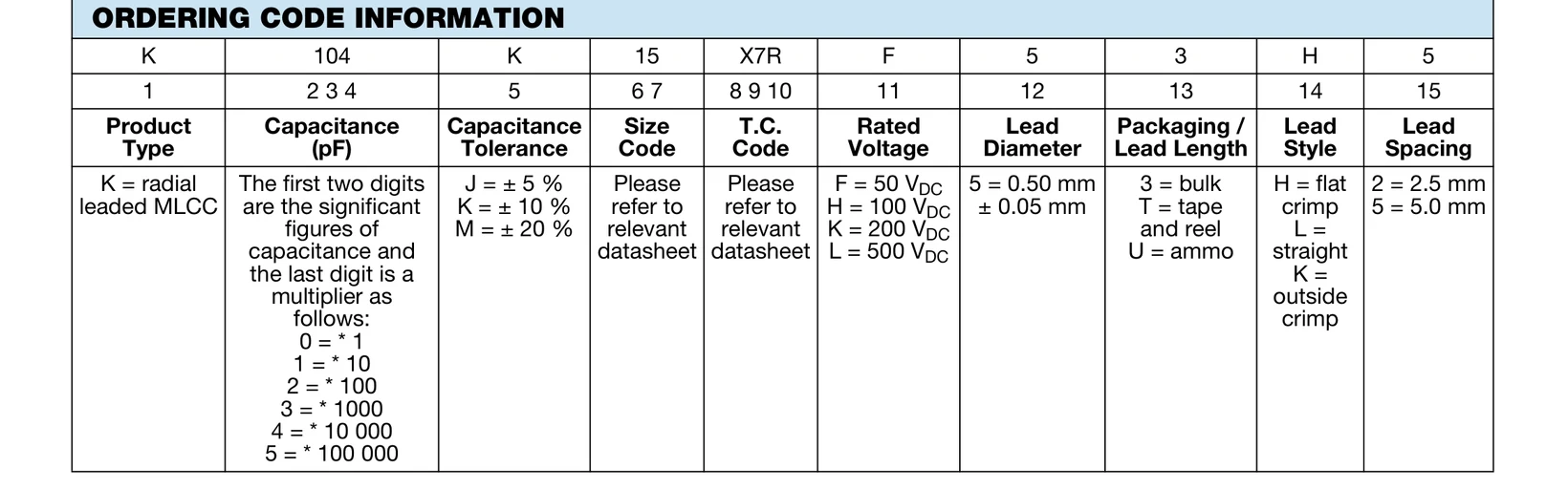
Vishay K series radial ceramic capacitors, document 45171, p. 2. The code on the part is the same as in the part number.
Is the part in tolerance?
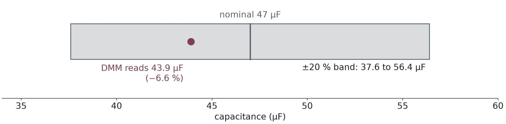
A 47 µF, ±20 % electrolytic may read anywhere from 37.6 to 56.4 µF. Discharge it and take it out of the circuit before you measure.
Part 2 · A time-dependent signal
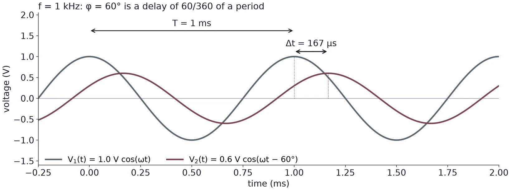
A phase is a time shift: . Here 60° of a 1 ms period is 167 µs.
Complex form and Euler's formula
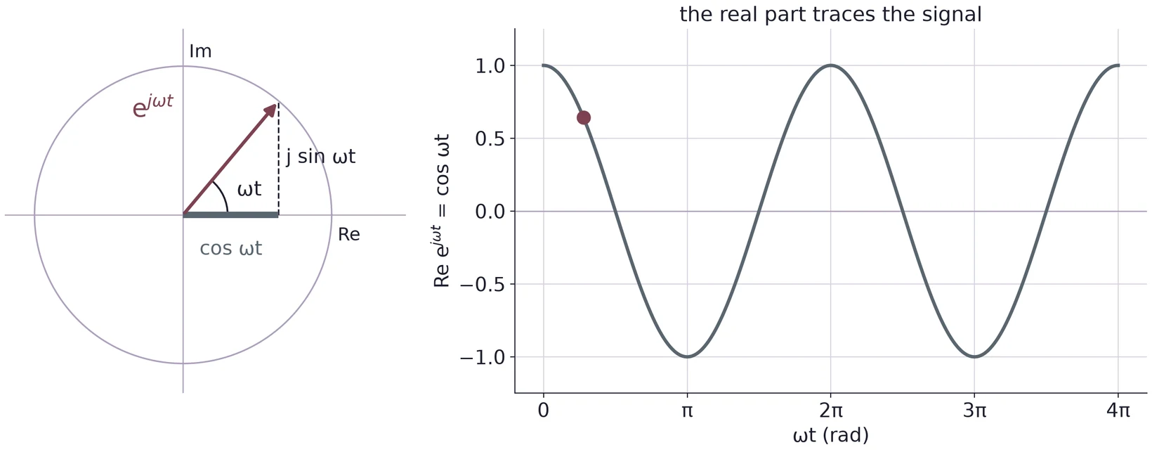
; we write because is the current. The voltage you measure is the real part. may be complex: it holds the amplitude and the phase.
The current into a capacitor: I = C dV/dt
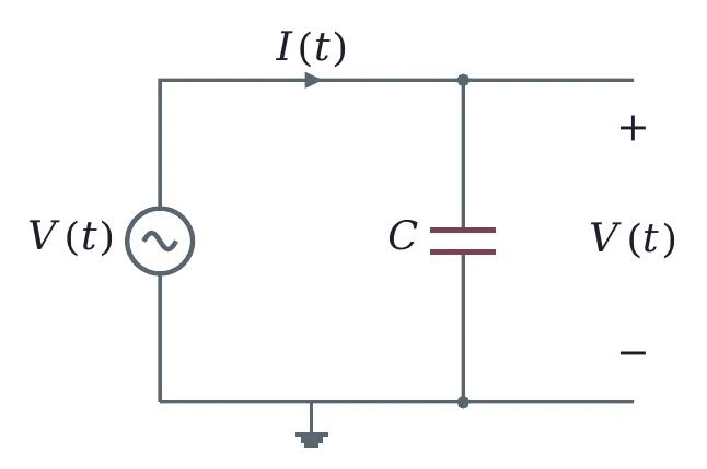
With :
holds only for a constant current. A changing current needs .
Worked: 1 µF, 5 V, 60 Hz
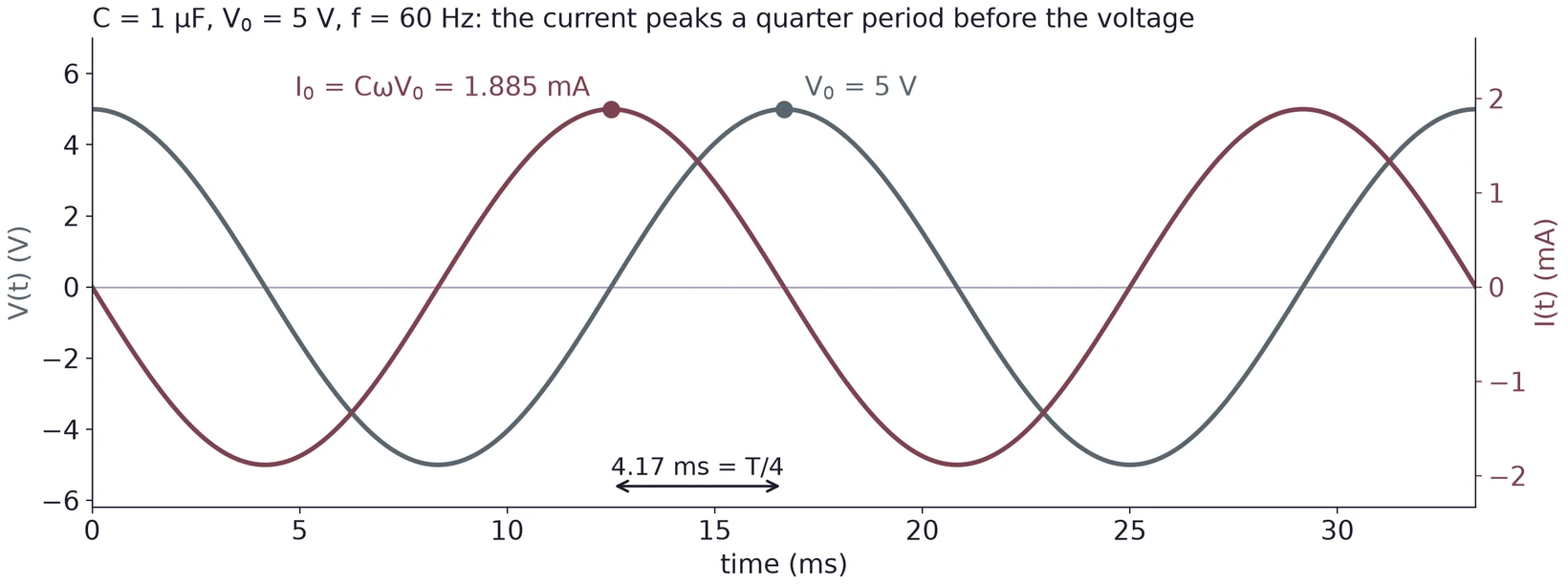
The current leads the voltage by 90°
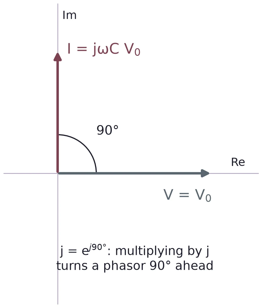
Same frequency, times the size, 90° ahead.
The current is largest when crosses zero, where changes fastest.
Part 3 · Impedance: Z = V/I
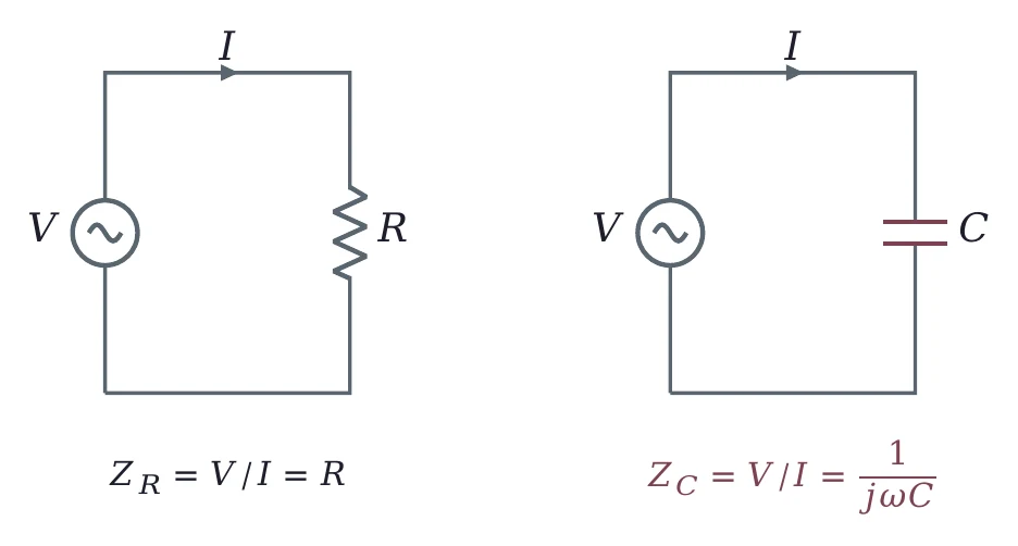
cancels, so does not depend on . Write or , never .
Reactance falls as frequency rises
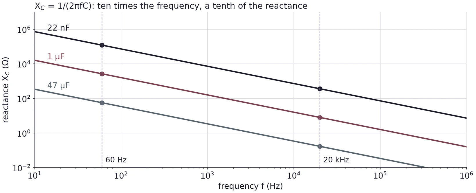
A capacitor blocks DC and slow signals and passes fast ones. A larger capacitor passes lower frequencies.
R and C in series: the impedance triangle
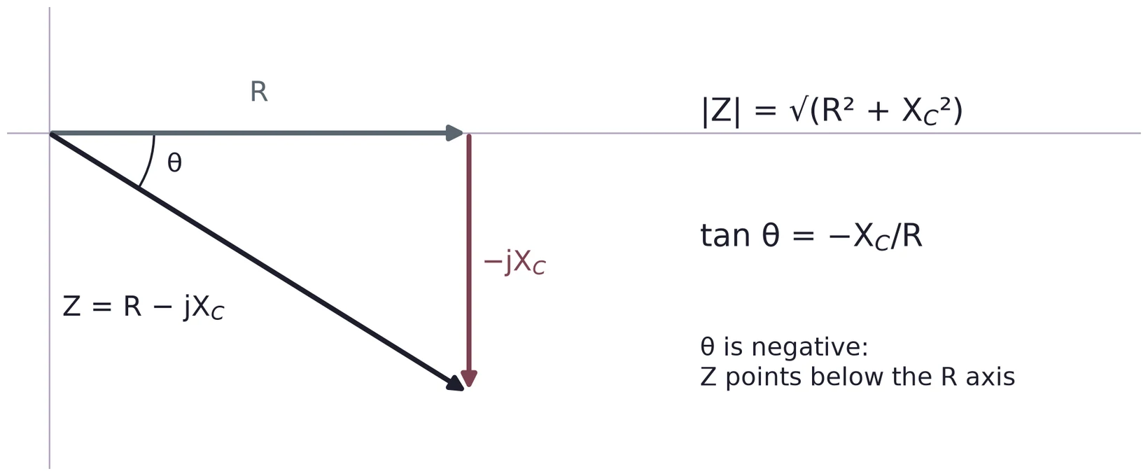
Worked: 3.3 kΩ and 10 nF at 10 kHz
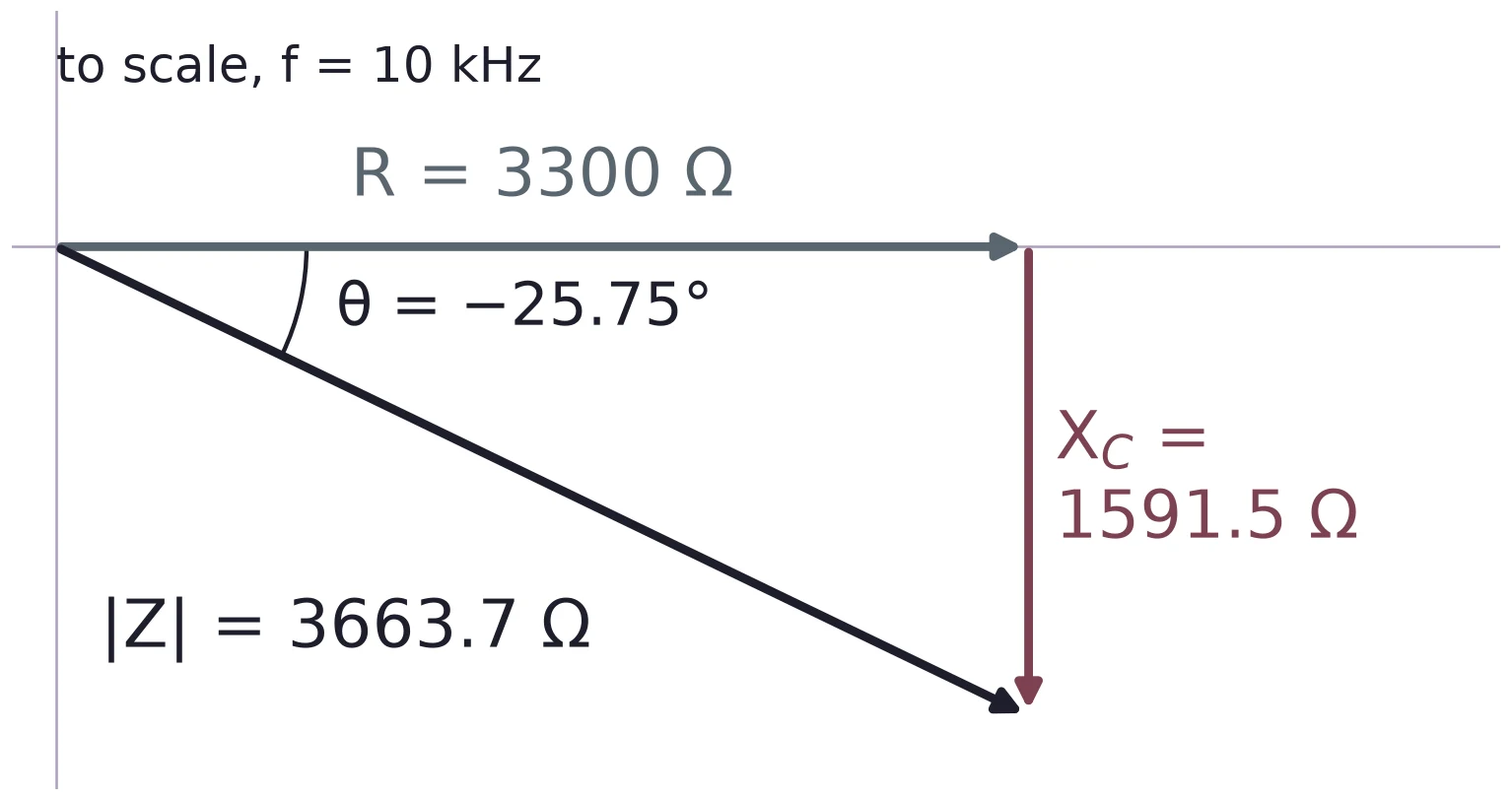
The angle is measured from the R axis, so . gives 64.25°, the other angle of the triangle.
Part 4 · A divider with a capacitor
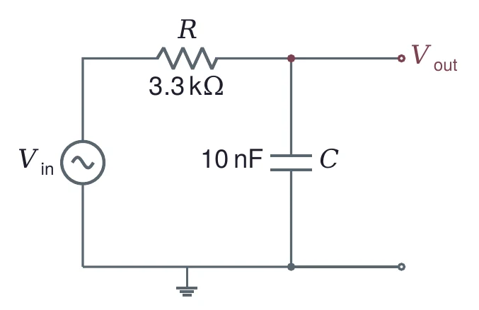
Low : is large, C is nearly open: .
High : is small, C is nearly a short: .
The divider of Lecture 01 with in place of . It passes low frequencies: a low-pass filter.
The transfer function
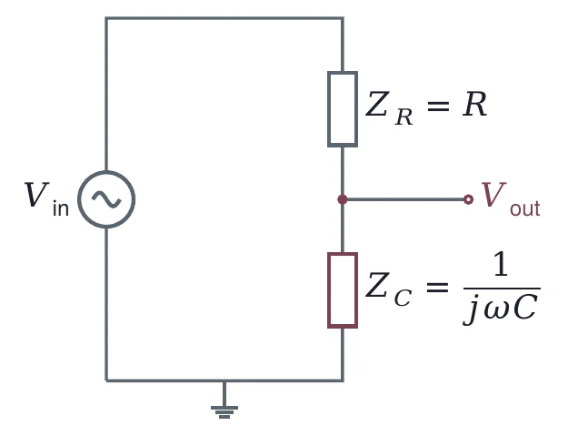
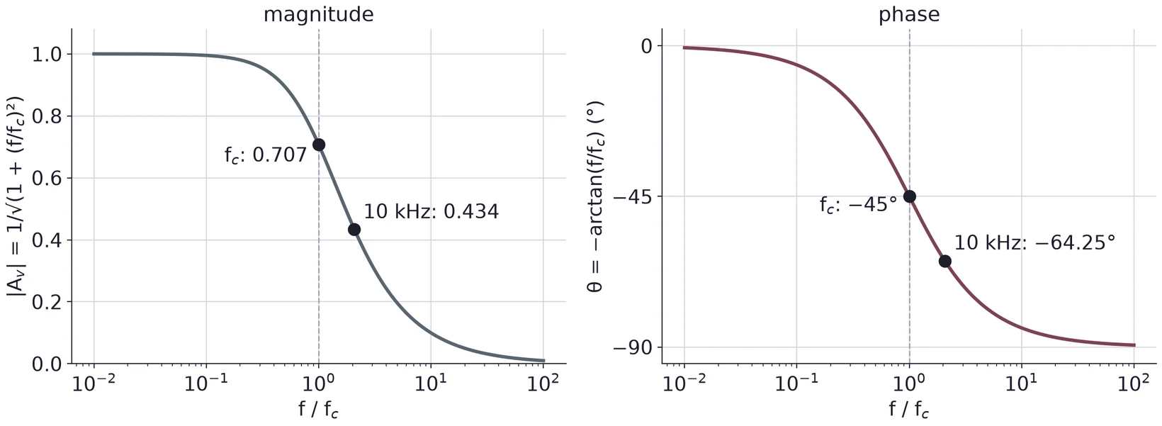
Use the complex . With magnitudes, would give 0.5 at cutoff instead of 0.707.
Cutoff: ωc = 1/RC
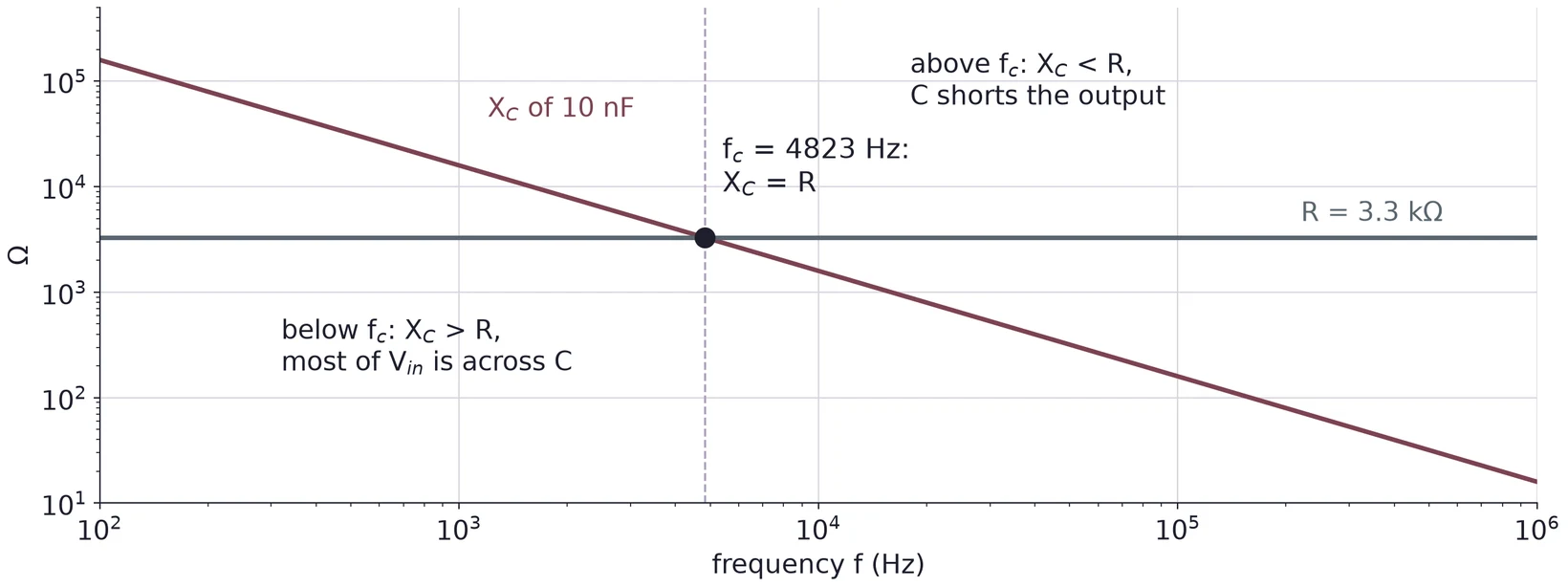
= 33 µs and = 30 303 rad/s, so . At the reactance equals .
Magnitude and phase in polar form
The Bode plot
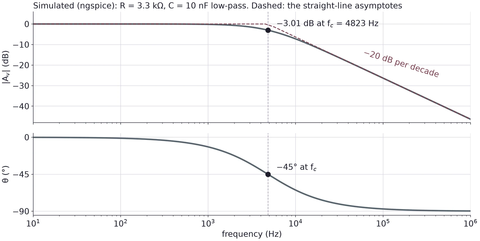
Simulated in ngspice. Above the gain falls 20 dB per decade (6.02 dB per octave), and the phase heads for −90°.
A Bode table for the 4.82 kHz low-pass
| f | |Av| | dB | θ |
|---|---|---|---|
| fc/20 | 0.9988 | −0.01 | −2.86° |
| fc/3 | 0.9487 | −0.46 | −18.43° |
| fc | 0.7071 | −3.01 | −45.00° |
| 3fc | 0.3162 | −10.00 | −71.57° |
| 20fc | 0.0499 | −26.03 | −87.14° |
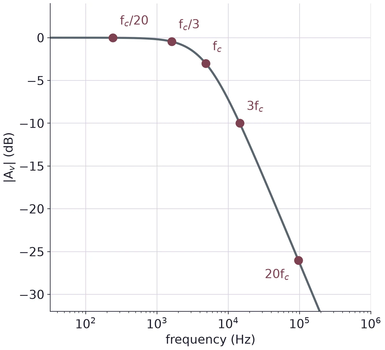
Only matters: is 1608 Hz here, is 14.47 kHz.
Part 5 · Swap R and C: the high-pass
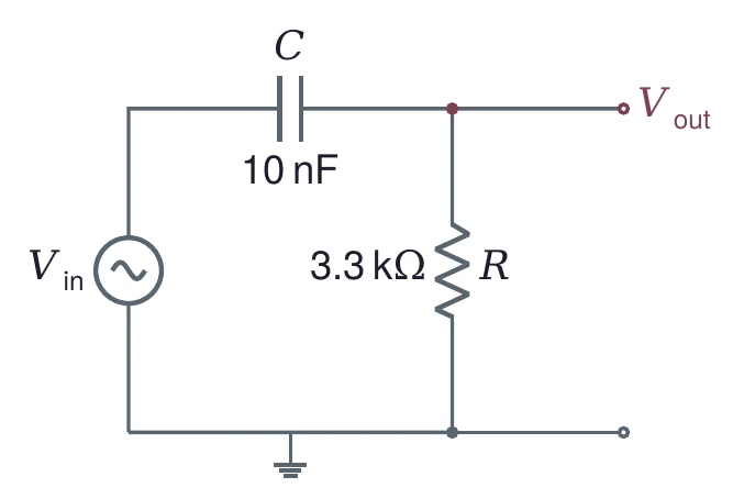
Same , but now the output is across R: low frequencies are blocked.
Designing for a cutoff
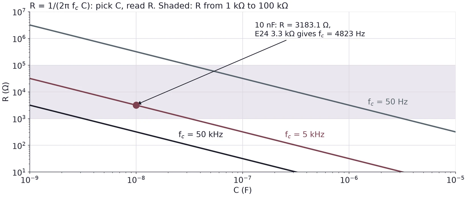
Pick C, compute R, round to a standard value, recompute . For 5 kHz with 10 nF: = 3183.1 Ω, E24 gives 3.3 kΩ, so = 4823 Hz.
Low-pass and high-pass on one Bode plot
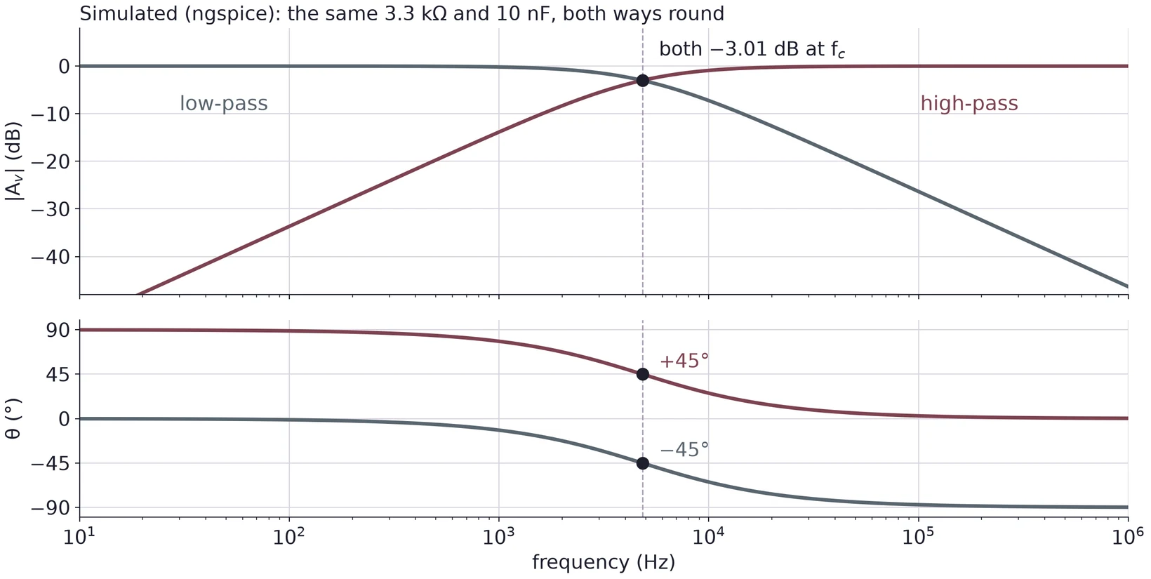
Simulated in ngspice. The high-pass at passes 0.3162 at +71.57°, as the low-pass does at with −71.57°.
Worked: the high-pass at 300 Hz, 1.0 Vpp in
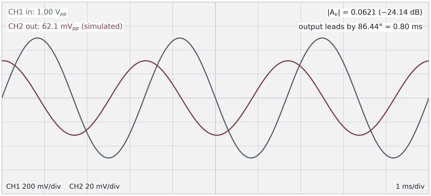
Out: 62.1 mV peak to peak, 31.0 mV peak, leading by 0.80 ms. Simulated in ngspice.
Part 6 · CH1 on the input, CH2 on the output
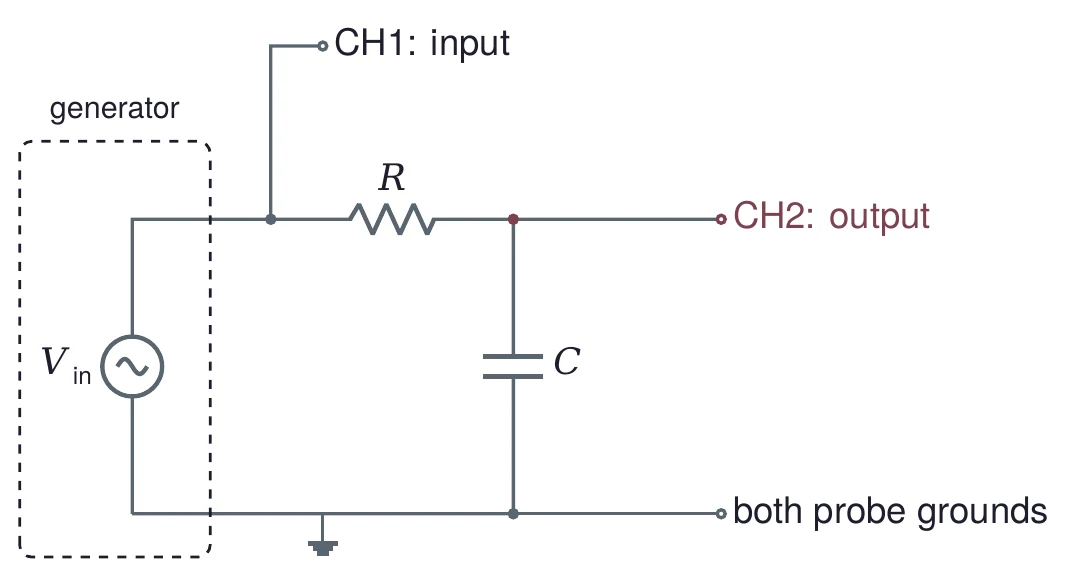
Both probe grounds go to circuit ground. Trigger on CH1, and read both channels at every frequency.
Finding fc: sweep until Vout = 0.707 Vin
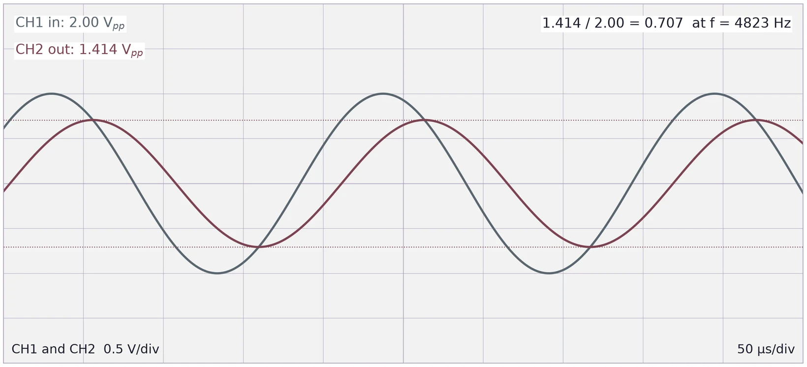
Watch the ratio, not alone. The filter loads the generator's 50 Ω differently at each frequency, so can move a little too.
Phase from the time shift
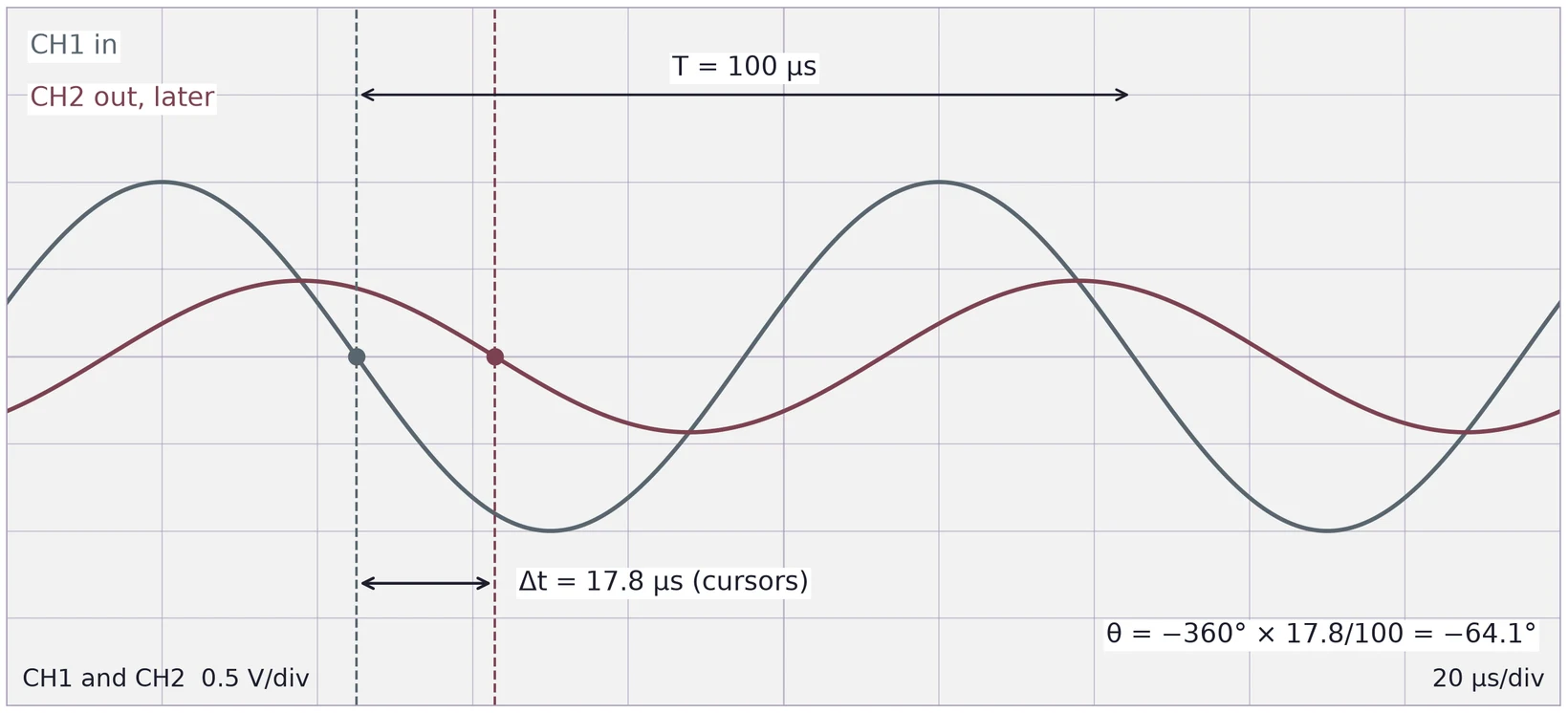
. At 10 kHz theory gives −64.25°, a delay of 17.85 µs. A cursor reading of 17.8 µs gives −64.08°.
From measurements to a Bode plot
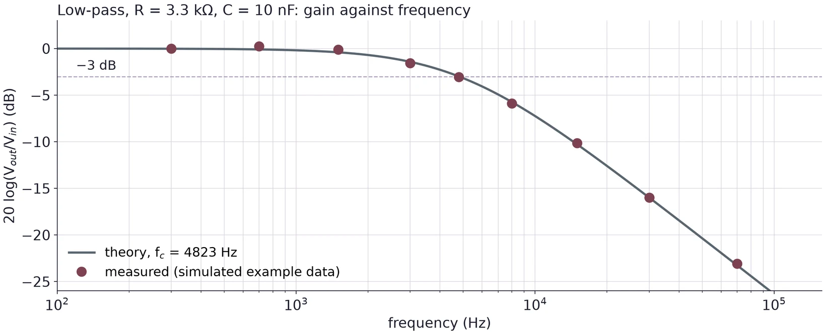
Plot against on a log axis, with the theory curve. Label which points are measured.
Error analysis in every task
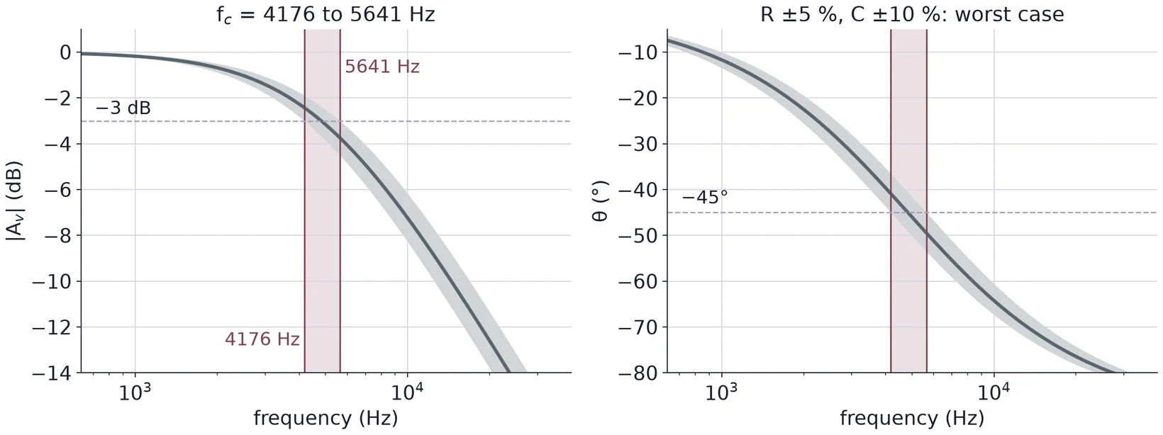
R ±5 % and C ±10 % move by ±11.2 % in quadrature, or from 4176 to 5641 Hz in the worst case. Near , a 1 % error in is a 2.0 % error in ; a 1° phase error is 3.5 %.
Use ← → to move, Home / End to jump, and F for fullscreen.
Figure descriptions
Slide 2 · Part 1 · Lab 3 in five tasks
Lab 3 in three rows. Know the parts: Task 1, measure three capacitors and find their reactance. Build a filter: Task 2, design a high-pass filter and drive it at 20 Hz. Measure it: Task 3, find the cutoff frequency and the gain there, then Task 4, the phase at the cutoff, then Task 5, seven points for a Bode plot.
Slide 3 · A capacitor stores charge
A sketch of a parallel-plate capacitor connected to a battery V. The top plate carries plus signs and the label +Q; the bottom plate carries minus signs and the label minus Q. An insulator fills the gap, with field arrows pointing from the top plate to the bottom one. Below: Q = CV.
Slide 4 · Polarized and non-polarized
Assorted capacitors on a gray background: large and small blue and black aluminum electrolytic cans marked with microfarads and volts, a metal-cased paper capacitor, orange and blue ceramic discs marked 103K, 151, 561 and 10, a green film capacitor marked 224K 100V, and two variable capacitors with ceramic frames.
Two capacitor symbols. Left, non-polarized (ceramic, film): two straight parallel plates. Right, polarized (electrolytic, tantalum): one curved plate and one straight plate, with a plus sign on the straight side.
Slide 5 · Three kinds side by side
A close-up row of small capacitors: a blue ceramic disc marked 561, small orange ceramic discs, a green film capacitor marked 224K 100V, a larger orange ceramic disc marked 103K 500V, and a small black electrolytic capacitor marked 22 microfarads 35 V.
Slide 6 · The electrolytic datasheet
Specifications table from the Nichicon UVR aluminum electrolytic capacitor datasheet: category temperature range minus 40 to plus 85 degrees C; rated voltage 6.3 to 450 V; rated capacitance 1 to 22000 microfarads; capacitance tolerance plus or minus 20 percent at 120 Hz and 20 degrees C; leakage current limits; and the maximum tangent of loss angle, tan delta, for each rated voltage, from 0.28 at 6.3 V to 0.08 at 100 V.
Slide 7 · Reading a ceramic code: 104K
Ordering code table from the Vishay K series ceramic capacitor datasheet, using the example K104K15X7RF53H5. Position 1, K, is the product type. Positions 2 to 4, 104, are the capacitance in picofarads: two significant digits and a multiplier digit. Position 5 is the tolerance: J for 5 percent, K for 10 percent, M for 20 percent. Then the size code, the dielectric (X7R), the rated voltage code (F for 50 V, H for 100 V, K for 200 V, L for 500 V), lead diameter, packaging, lead style and lead spacing.
Slide 8 · Is the part in tolerance?
A capacitance axis from 34 to 60 microfarads. A shaded band from 37.6 to 56.4 microfarads is the plus or minus 20 percent tolerance of a 47 microfarad capacitor, marked at its nominal value. A DMM reading of 43.9 microfarads, minus 6.6 percent, lies inside the band.
Slide 9 · Part 2 · A time-dependent signal
Two sine waves at 1 kHz plotted against time from minus 0.25 to 2 ms. V1 is 1.0 V cos(omega t); V2 is 0.6 V cos(omega t minus 60 degrees), smaller and shifted later. Arrows mark the period T = 1 ms and the delay of 167 microseconds between a peak of V1 and the next peak of V2.
Slide 10 · Complex form and Euler's formula
Left: a unit circle with a rotating arrow e to the j omega t at angle omega t from the real axis; its projection on the real axis is cos omega t and its height is j sin omega t. Right: cos omega t plotted against omega t from 0 to 4 pi, with a dot at the angle of the arrow, showing that the real part traces the signal.
Slide 11 · The current into a capacitor: I = C dV/dt
An AC source V(t) connected directly across a capacitor C, with the current I(t) flowing from the source into the capacitor and the voltage V(t) marked across it. The bottom wire is grounded.
Slide 12 · Worked: 1 µF, 5 V, 60 Hz
Voltage and current of a 1 microfarad capacitor driven by 5 V at 60 Hz, plotted against time for two periods (33.3 ms). The voltage, left axis, peaks at 5 V. The current, right axis, peaks at 1.885 mA a quarter period (4.17 ms) before each voltage peak.
Slide 13 · The current leads the voltage by 90°
A phasor diagram. The voltage phasor V = V0 lies along the real axis. The current phasor I = j omega C V0 points straight up along the imaginary axis, 90 degrees ahead. A note says that multiplying by j turns a phasor 90 degrees ahead.
Slide 14 · Part 3 · Impedance: Z = V/I
Two circuits side by side. Left: a source V drives current I through a resistor R, with Z_R = V/I = R. Right: a source V drives current I through a capacitor C, with Z_C = V/I = 1/(j omega C).
Slide 15 · Reactance falls as frequency rises
Capacitive reactance against frequency from 10 Hz to 1 MHz on log-log axes for 47 microfarads, 1 microfarad and 22 nanofarads: three parallel straight lines falling a factor of ten per decade. Dashed lines at 60 Hz and 20 kHz mark the worked values.
Slide 17 · R and C in series: the impedance triangle
The impedance triangle of a series RC circuit. R points right along the real axis; from its tip, minus j X_C points straight down; the hypotenuse Z = R minus j X_C points down and to the right at angle theta below the R axis. Beside it: the magnitude of Z equals the square root of R squared plus X_C squared, tan theta = minus X_C over R, and theta is negative.
Slide 18 · Worked: 3.3 kΩ and 10 nF at 10 kHz
The impedance triangle drawn to scale for 3.3 kilohms and 10 nanofarads at 10 kHz: R = 3300 ohms along the real axis, X_C = 1591.5 ohms downward, the magnitude of Z = 3663.7 ohms, and theta = minus 25.75 degrees.
Slide 19 · Part 4 · A divider with a capacitor
An RC low-pass filter: the source V_in drives a 3.3 kilohm resistor R in series with a 10 nanofarad capacitor C to ground; the output V_out is taken across the capacitor.
Slide 20 · The transfer function
A voltage divider made of two impedance boxes: Z_R = R on top and Z_C = 1/(j omega C) below, driven by V_in, with V_out taken at the node between them.
Slide 21 · Cutoff: ωc = 1/RC
Reactance of a 10 nanofarad capacitor and a 3.3 kilohm resistance against frequency from 100 Hz to 1 MHz on log-log axes. The falling reactance line crosses the flat R line at f_c = 4823 Hz, where X_C = R. Below f_c, X_C is larger than R and most of V_in is across C; above f_c, X_C is smaller than R and C shorts the output.
Slide 22 · Magnitude and phase in polar form
Two plots against f over f_c on a log axis from 0.01 to 100. Left, magnitude: 1/sqrt(1 + (f/f_c) squared), flat at 1, then falling, with 0.707 marked at f_c and 0.434 at 10 kHz. Right, phase: minus arctan(f/f_c), from 0 to minus 90 degrees, with minus 45 degrees at f_c and minus 64.25 degrees at 10 kHz.
Slide 24 · The Bode plot
Simulated Bode plot from ngspice of the 3.3 kilohm, 10 nanofarad low-pass, 10 Hz to 1 MHz. Top: gain in dB, flat at 0 dB, minus 3.01 dB at f_c = 4823 Hz, then falling at minus 20 dB per decade, with dashed straight-line asymptotes. Bottom: phase from 0 to minus 90 degrees, minus 45 degrees at f_c.
Slide 25 · A Bode table for the 4.82 kHz low-pass
The gain in dB of the 4823 Hz low-pass against frequency, with five points marked: f_c/20 near 0 dB, f_c/3 at minus 0.46 dB, f_c at minus 3.01 dB, 3 f_c at minus 10.00 dB and 20 f_c at minus 26.03 dB.
Slide 26 · Part 5 · Swap R and C: the high-pass
An RC high-pass filter: the source V_in drives a 10 nanofarad capacitor C in series with a 3.3 kilohm resistor R to ground; the output V_out is taken across the resistor.
Slide 27 · Designing for a cutoff
A design chart on log-log axes: resistance R from 10 ohms to 10 megohms against capacitance C from 1 nanofarad to 10 microfarads. Three falling lines show the pairs that give f_c = 50 Hz, 5 kHz and 50 kHz. A shaded band marks R from 1 kilohm to 100 kilohms. A marked point at 10 nanofarads: the exact R is 3183.1 ohms, and the E24 value 3.3 kilohms gives f_c = 4823 Hz.
Slide 28 · Low-pass and high-pass on one Bode plot
Simulated Bode plots from ngspice of the low-pass and the high-pass built from the same 3.3 kilohms and 10 nanofarads. Top: the low-pass gain is flat then falls; the high-pass gain rises then is flat; they cross at f_c, both at minus 3.01 dB. Bottom: the low-pass phase goes from 0 to minus 90 degrees and the high-pass phase from plus 90 to 0 degrees, minus 45 and plus 45 degrees at f_c.
Slide 29 · Worked: the high-pass at 300 Hz, 1.0 Vpp in
A simulated two-channel scope screen at 1 ms per division. CH1 at 200 mV per division shows the 1.00 V peak-to-peak, 300 Hz input. CH2 at 20 mV per division shows the high-pass output, 62.1 mV peak-to-peak, leading the input by 86.44 degrees, 0.80 ms. The gain is 0.0621, minus 24.14 dB.
Slide 30 · Part 6 · CH1 on the input, CH2 on the output
Measuring a filter on the scope: a generator V_in drives R then C to ground. CH1 connects to the input node before R, CH2 to the output node between R and C, and both probe grounds connect to the circuit ground.
Slide 31 · Finding fc: sweep until Vout = 0.707 Vin
A scope screen at 0.5 V per division and 50 microseconds per division with the low-pass at f = 4823 Hz. CH1, the input, is 2.00 V peak to peak; CH2, the output, is 1.414 V peak to peak and slightly later. Dotted lines mark the output peaks. The ratio 1.414 over 2.00 is 0.707.
Slide 32 · Phase from the time shift
A scope screen at 0.5 V per division and 20 microseconds per division with the low-pass at 10 kHz. Dashed cursors mark the falling zero crossings of the input (CH1) and the smaller output (CH2); the output crosses 17.8 microseconds later. One period is 100 microseconds, so theta = minus 360 degrees times 17.8/100 = minus 64.1 degrees.
Slide 33 · From measurements to a Bode plot
A report Bode plot: gain in dB, 20 log of V_out over V_in, against frequency from 100 Hz to about 160 kHz on a log axis. The theory curve of the low-pass with f_c = 4823 Hz, and nine measured points from simulated example data that lie close to it, with a dashed line at minus 3 dB.
Slide 34 · Error analysis in every task
Two plots near the cutoff of the 4823 Hz low-pass. With R plus or minus 5 percent and C plus or minus 10 percent, the gain curve (left) and the phase curve (right) can lie anywhere in a shaded band, and the cutoff can lie anywhere from 4176 to 5641 Hz, marked by two vertical lines. Dashed lines mark minus 3 dB and minus 45 degrees.