1 Where Lab 3 Sits
Lab 3 brings a new part to the bench: the capacitor. First you measure three capacitors and work out how they behave at a low and a high frequency. Then you build one filter from a resistor and a capacitor, and you measure how it treats each frequency: where it cuts off, how much it shifts the phase, and its full Bode plot.
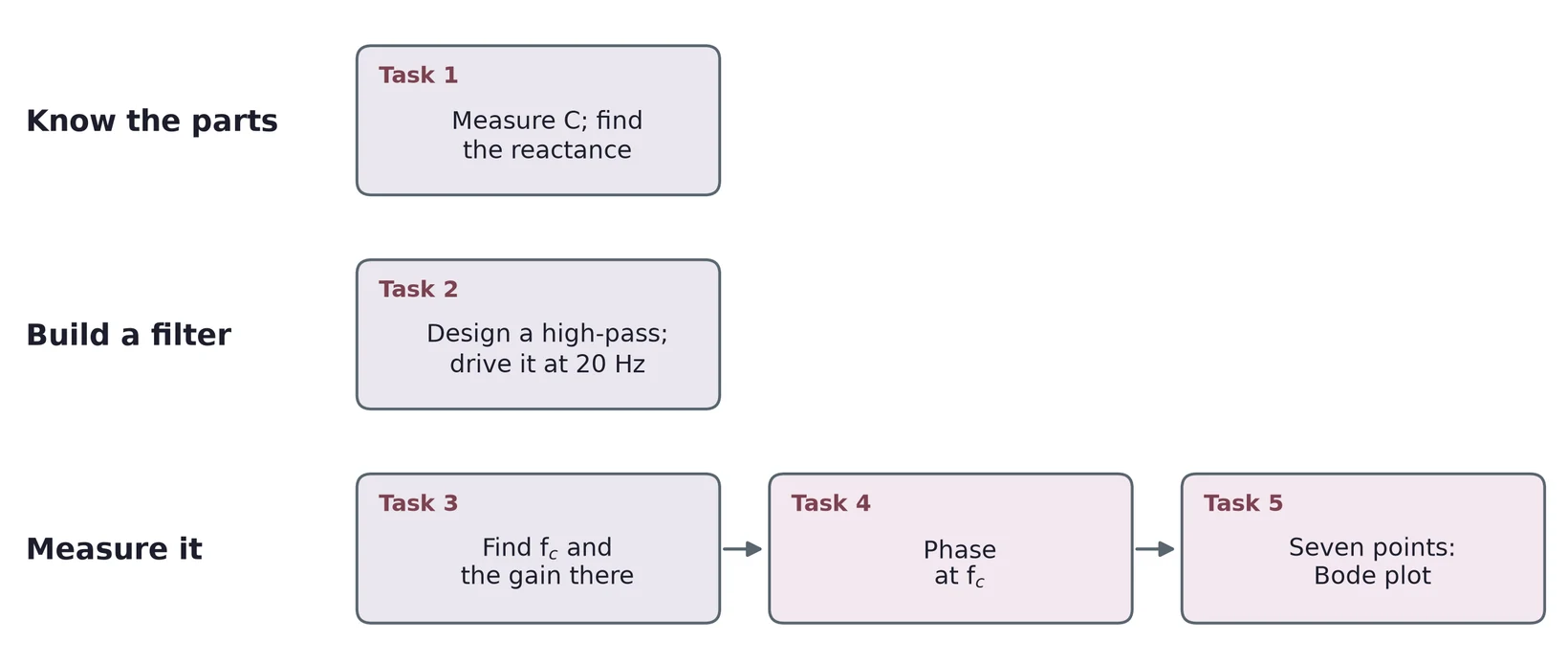
1.1 Task map
| Lab 3 task | What you do | Concept & section |
|---|---|---|
| 1 | Measure three capacitors; compare polarized and unpolarized; find their reactance at two frequencies | Capacitors (§2), reactance (§4) |
| 2 | Design and build a high-pass filter; drive it at a low frequency | The low-pass (§5), the high-pass and design (§6) |
| 3 | Measure the cutoff frequency; find the gain there in V/V and in dB | Cutoff and decibels (§5), finding on the scope (§7) |
| 4 | Measure the phase at the cutoff; compare with calculation and simulation | Phase (§3, §5), phase from a time shift (§7) |
| 5 | Measure seven points and draw a Bode plot | The Bode plot (§5, §6), from data to a plot (§7) |
Every task needs an error analysis. Section 8 collects the main error sources for each kind of measurement.
2 Capacitors
2.1 A capacitor stores charge
A capacitor is two conductors separated by an insulator. Connect it to a voltage and charge flows until one plate holds and the other . No charge crosses the insulator; the charge on one plate pushes the same amount off the other. The charge is proportional to the voltage:
The constant is the capacitance, in farads (F). One farad stores one coulomb per volt, which is a lot: the parts on your bench run from picofarads ( F) to a few thousand microfarads ( F).
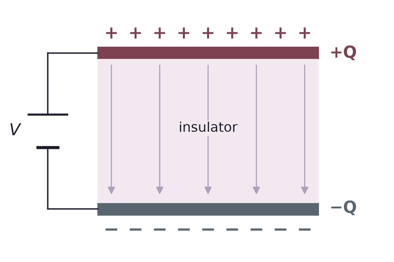
At 9 V, a 47 µF capacitor holds C, or 423 µC.
2.2 Polarized and non-polarized
Capacitors come in two families. A non-polarized capacitor, such as a ceramic or film part, works with either lead at the higher voltage. A polarized capacitor, such as an aluminum electrolytic or a tantalum part, has a + lead that must stay at the higher voltage.
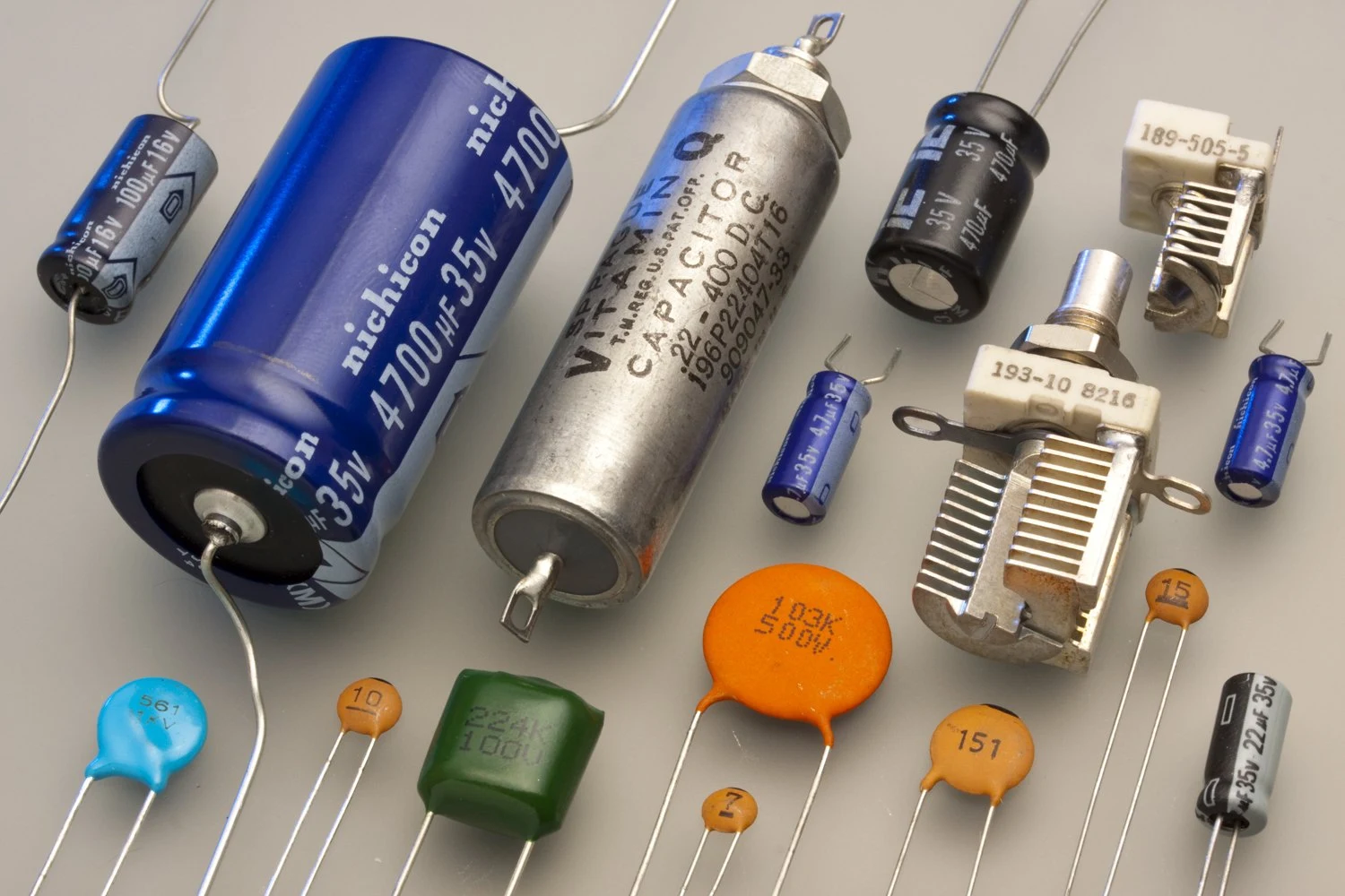

The reason is in how an electrolytic is made. Its insulator is a thin oxide layer grown on aluminum foil. A thin insulator gives a large capacitance in a small can, but the oxide holds only while the foil is positive. Reverse the voltage and a leakage current flows through it: the part heats up and can bulge or vent. The can is marked with a stripe on the − side, and the − lead is usually the shorter one.
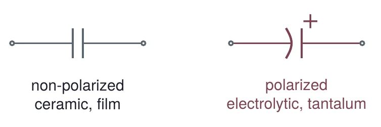
2.3 Three kinds side by side
The table compares one common series of each kind. Each row comes from that series' datasheet.
| Kind (series) | Range | Tolerance | Polarized? | Used for |
|---|---|---|---|---|
| Aluminum electrolytic (Nichicon UVR) | 1 to 22 000 µF | ±20 % | yes | large values: smoothing a supply, storing charge |
| Ceramic, C0G or X7R (Vishay K series) | 10 pF to 1 µF | ±5, 10 or 20 % | no | coupling and decoupling; C0G for stable values |
| Film, polyester (WIMA MKS 2) | 0.01 to 4.7 µF | ±5, 10 or 20 % | no | coupling, decoupling, timing |
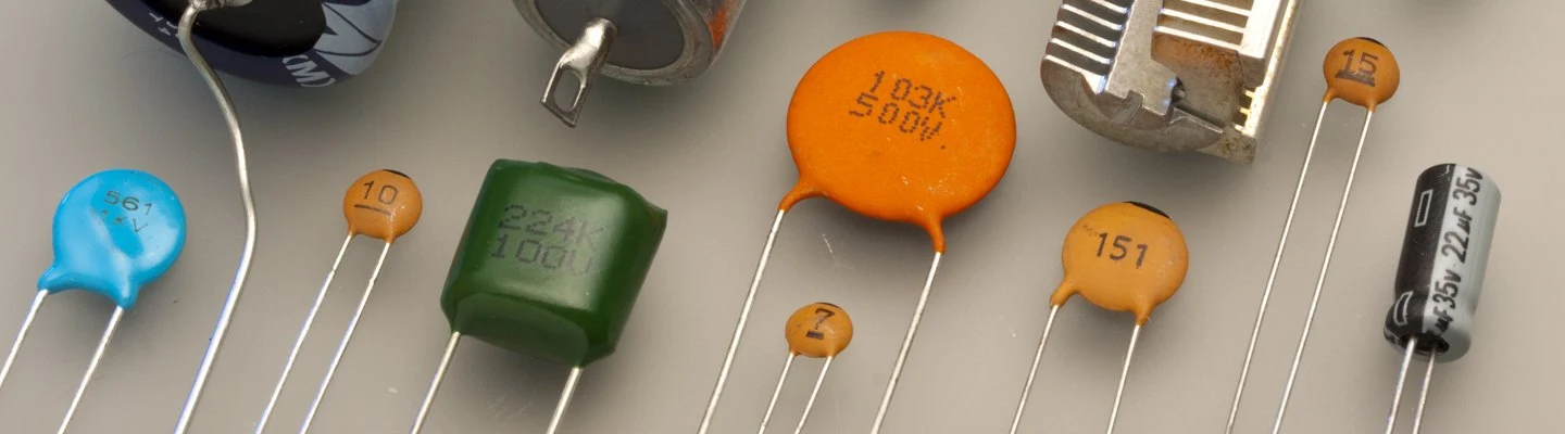
C0G ceramics keep their value over temperature. X7R ceramics pack more capacitance into the same size, but their value drifts more with temperature and with the voltage across them. Film parts sit in between and stay close to their value.
2.4 Reading the datasheet
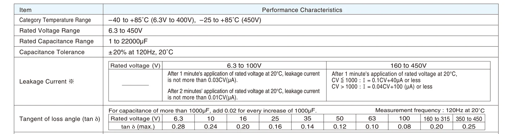
Figure 6 is the specification table of a common electrolytic series. Three lines matter here. The rated voltage is the most you may put across the part. The capacitance tolerance is ±20 %, measured at 120 Hz and 20 °C. The tangent of the loss angle, tan δ, measures the loss: it is the ratio of the part's internal series resistance to its reactance (§4), so a perfect capacitor has tan δ = 0. For this series it runs from 0.28 for 6.3 V parts down to 0.08 for 100 V parts.
Small ceramic and film parts are too small for a written value, so they carry a three-digit code in picofarads: two digits, then the number of zeros. A letter after it gives the tolerance: J = ±5 %, K = ±10 %, M = ±20 %. Figure 7 shows the same code inside a part number.
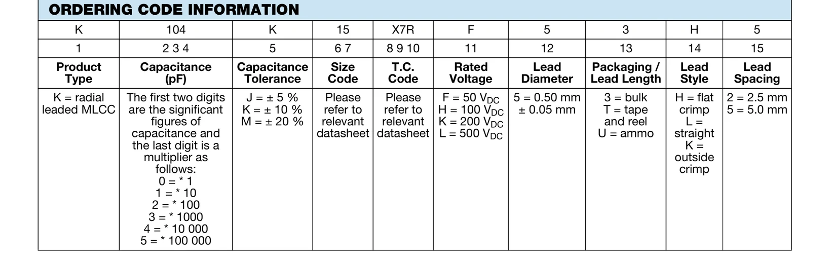
The digits 1, 0 and then four zeros give 100 000 pF = 100 nF = 0.1 µF. K means ±10 %.
A code under 100 is the value itself in picofarads: a disc marked 15 is 15 pF.
2.5 Measuring C and checking the tolerance
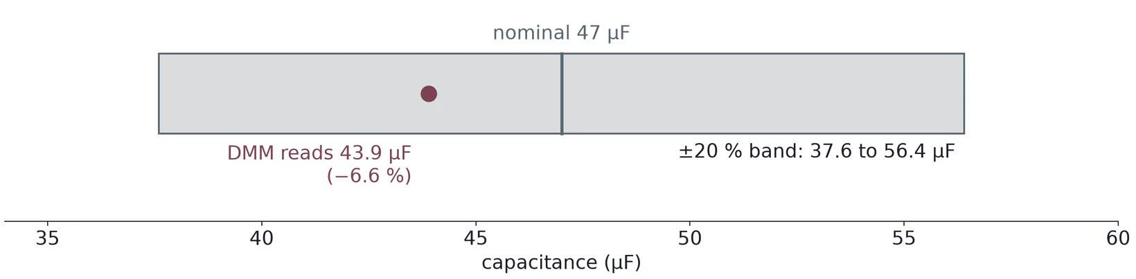
Many DMMs have a capacitance range. Take the capacitor out of the circuit and discharge it first: short its leads through a resistor, since a charged electrolytic can damage the meter's input. Then compare the reading with the nominal value, as you did for resistors in Lab 1:
The DMM reads 43.9 µF. The deviation is (43.9 − 47)/47 × 100 % = −6.60 %. A ±20 % part may lie anywhere from 0.8 × 47 = 37.6 µF to 1.2 × 47 = 56.4 µF, so this one is in tolerance.
The meter's capacitance range has its own accuracy, usually a few percent plus some counts, and it is often worse on the smallest ranges. Look it up in your meter's manual for the range you used.
(a) How much charge does a 220 µF capacitor hold at 12 V?
(b) A film capacitor is marked 224K. What are its nominal value and its tolerance range?
(c) A 220 µF, ±20 % electrolytic reads 241 µF. What is the deviation? Is it in tolerance?
(d) Why must an electrolytic's + lead go to the higher voltage?
3 AC Signals and the Capacitor's Current
3.1 A time-dependent signal
Until now every voltage stayed constant. In this lab the generator makes a sine wave, so the voltage changes with time:
is the amplitude, the frequency in hertz, the angular frequency in radians per second, and the phase. A phase is a shift in time. One period is 360°, so a phase of shifts the wave by
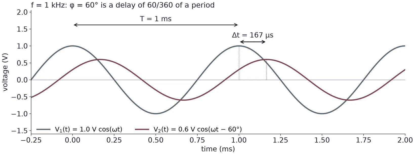
Two numbers describe how a circuit changes a sine wave: the ratio of the amplitudes and the phase shift. A circuit of resistors and capacitors never changes the frequency.
3.2 Complex form and Euler's formula
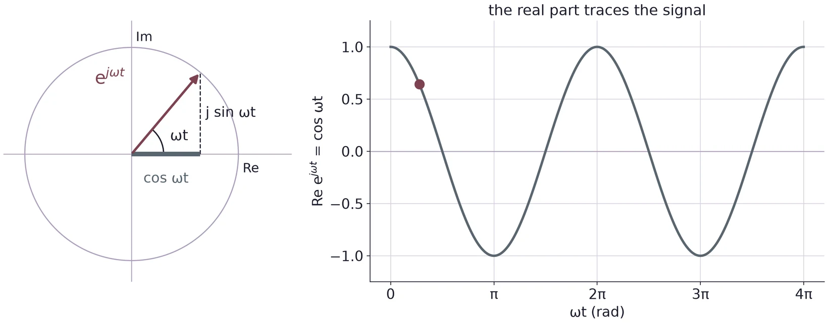
Sines are awkward to differentiate and add. Complex numbers make them easy. In electronics we write for , since is already the current. Euler's formula links an exponential to a cosine and a sine:
So we write the signal as
and keep in mind that the voltage you measure is its real part, . The number may be complex: its size is the amplitude and its angle is the phase.
3.3 The current into a capacitor
Drive a capacitor with . The charge follows the voltage, , and the current is the rate at which charge arrives:
The familiar holds only when the current is constant; here it is not, so we use the derivative.
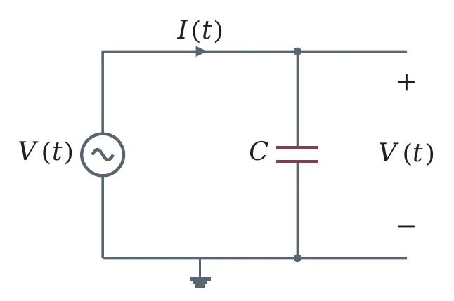
With the complex form, the derivative is one step. The derivative of is , so
The current has the same frequency as the voltage. Its amplitude is , and it grows with frequency: a capacitor lets more current through when the voltage changes faster.
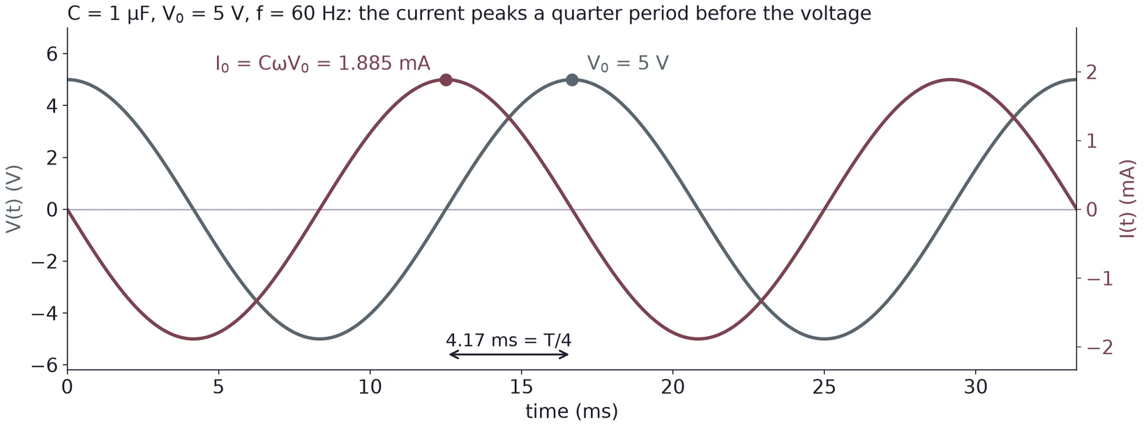
rad/s, so A = 1.885 mA. The period is 16.67 ms, and the current peaks a quarter period, 4.17 ms, before the voltage.
3.4 The current leads by 90°
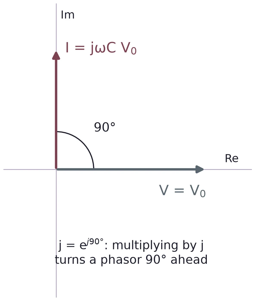
The factor in Equation (8) is a phase. Since , multiplying by turns a phasor 90° ahead. The current is therefore 90° ahead of the voltage: it peaks when the voltage crosses zero going up, where the voltage changes fastest, and it is zero at the voltage peaks, where the voltage stops changing for an instant.
(a) A 220 µF capacitor sits across a 120 Hz signal of 2 V amplitude. Find the amplitude of the current.
(b) For a 1 kHz signal, how long before the voltage peak does the capacitor's current peak?
(c) A sine at 2.5 kHz lags another by 40 µs. What is the phase shift in degrees?
(d) Why does give the wrong answer for a capacitor on a sine wave?
4 Impedance and Reactance
4.1 Z = V/I
For a resistor, . For a capacitor on a sine wave we do the same and divide Equation (6) by Equation (8). The result is the impedance:
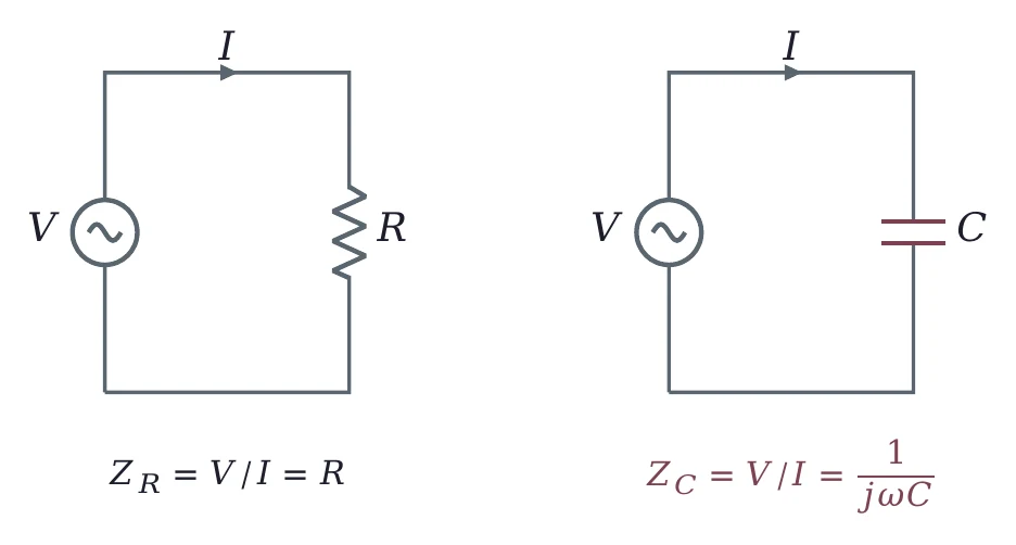
The factor cancels, so the impedance does not change with time. It changes with frequency: write or , not . Its size is the reactance,
measured in ohms. Keep the two apart. is a positive number of ohms; is complex and carries the 90° phase.
4.2 Reactance falls as frequency rises
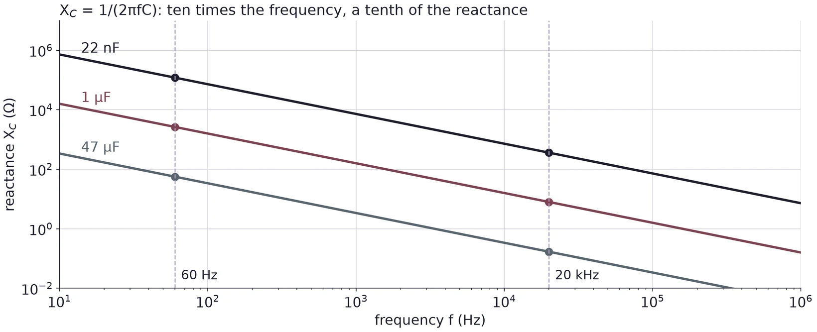
Equation (10) says is inversely proportional to both and . At DC ( = 0), is infinite: a capacitor blocks DC. At high frequency, is small: the capacitor acts almost like a wire. On log-log axes each capacitor gives a straight line that falls by a factor of ten per decade of frequency.
| Capacitor | at 60 Hz | at 20 kHz |
|---|---|---|
| 47 µF electrolytic | = 56.44 Ω | 0.1693 Ω |
| 1 µF film | = 2653 Ω | 7.958 Ω |
| 22 nF ceramic | = 120.6 kΩ | 361.7 Ω |
From 60 Hz to 20 kHz the frequency grows by 20 000/60 = 333.3, so each reactance shrinks by the same factor.
4.3 R and C in series: the impedance triangle
Impedances in series add, like resistors, but as complex numbers:
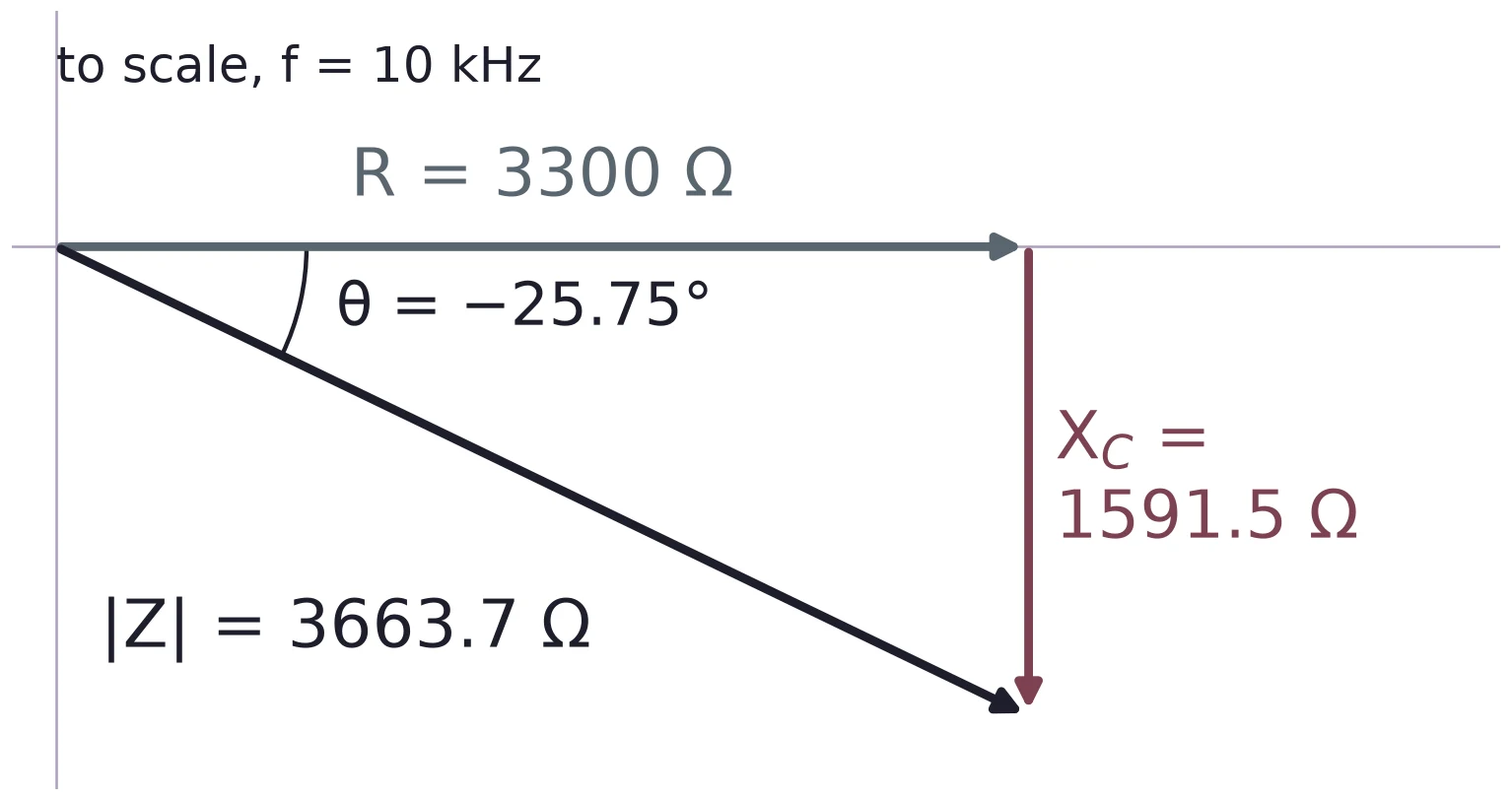
Draw along the real axis and straight down from its tip. The impedance is the hypotenuse of a right triangle:
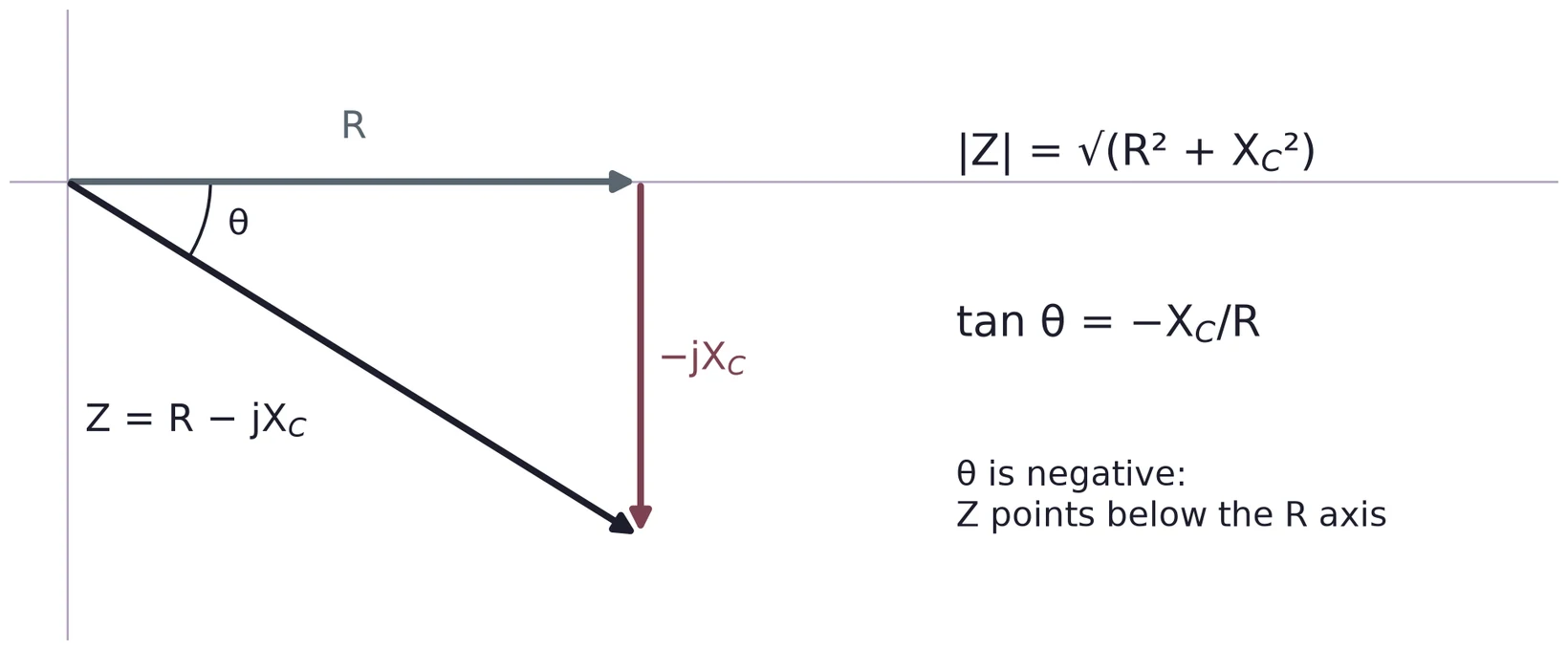
The angle is measured from the R axis, so the side opposite it is and the side next to it is . Writing gives the other acute angle of the triangle, the one at the tip of .
Ω. Ω. .
With you would get 64.25°, the complementary angle, which is not the angle of .
(a) Find the reactance of a 220 µF capacitor at 120 Hz.
(b) At what frequency does a 22 nF capacitor have a reactance of 1 kΩ?
(c) Find and for 10 kΩ in series with 1 nF at 40 kHz.
5 The RC Low-Pass Filter
5.1 A divider with a capacitor
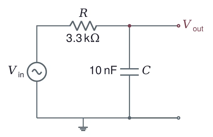
Put a capacitor in place of the lower resistor of a voltage divider and take the output across it. At low frequency is large, the capacitor is nearly an open circuit, and almost all of appears at the output. At high frequency is small, the capacitor is nearly a short, and the output falls toward zero. The circuit passes low frequencies and stops high ones: it is a low-pass filter.
5.2 The transfer function
The divider rule of Lecture 01 still holds, with impedances in place of resistances. The ratio of output to input is the voltage gain, also called the transfer function:
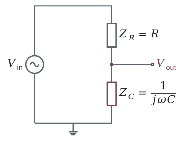
Use the complex in this step. The two impedances are 90° apart, so they do not add like numbers on a line. If you put the reactance into the divider instead, , you would get 0.5 at the cutoff instead of the correct 0.707.
5.3 The cutoff frequency
The product has units of time. It is the time constant , and its inverse is the cutoff:
With it, Equation (13) becomes
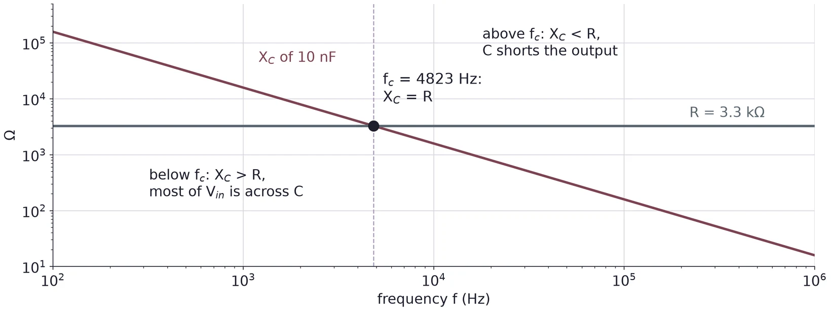
At the cutoff, , which is the same as . Below the capacitor's reactance is the larger one and most of the input appears across it; above the resistor takes most of it.
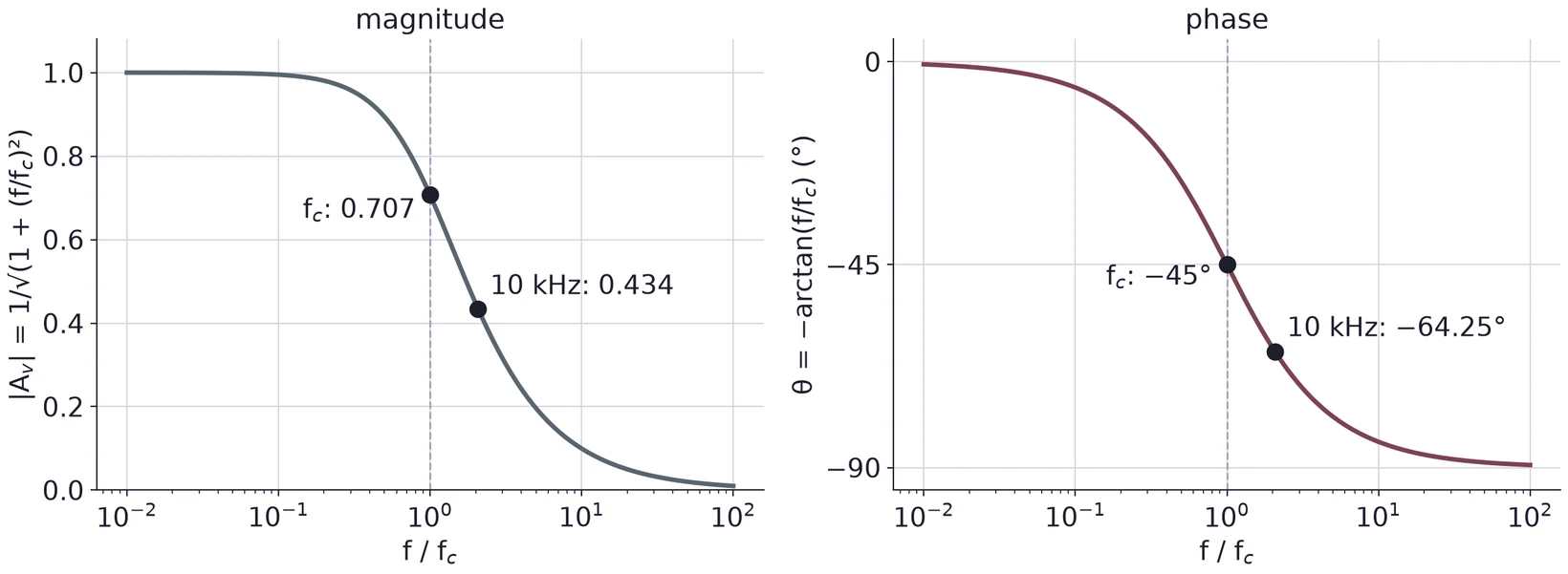
µs. rad/s. Hz, about 4.82 kHz. A simulation in ngspice puts the −3 dB point at the same 4822.9 Hz.
5.4 Magnitude and phase in polar form
A complex gain is easier to read in polar form, as a size times a phase. For , . With and , Equation (15) becomes
So the output amplitude is times the input amplitude, and the output lags the input by . At : and .
| 1 kHz | 0.2073 | 0.9792 | −11.71° |
| 4823 Hz | 1 | 0.7071 | −45.00° |
| 10 kHz | 2.073 | 0.4344 | −64.25° |
| 50 kHz | 10.37 | 0.0960 | −84.49° |
5.5 Decibels and the −3 dB point
Gains span many powers of ten, so we often give them in decibels:
A gain of 1 is 0 dB, 0.5 is −6.02 dB, 0.1 is −20 dB and 0.01 is −40 dB. For the low-pass, Equation (16) gives
At this is dB. That is why the cutoff is also called the −3 dB point. It holds for every first-order RC filter, whatever its R and C: only enters Equation (18). The same values in dB from the worked example above: −0.18 dB at 1 kHz, −7.24 dB at 10 kHz, −20.35 dB at 50 kHz.
5.6 The Bode plot
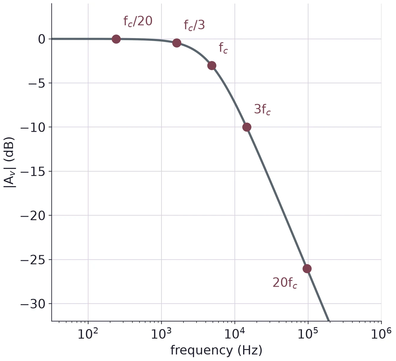
A Bode plot shows a filter's whole behavior in two graphs that share a log frequency axis: the gain in dB, and the phase in degrees. On these axes the low-pass looks like two straight lines joined by a bend. Far below the gain is 0 dB. Far above, , so : the gain falls 20 dB for every factor of ten in frequency (a decade), or 6.02 dB for every factor of two (an octave). The two straight lines, the asymptotes, meet at , where the real curve sits 3.01 dB below them.
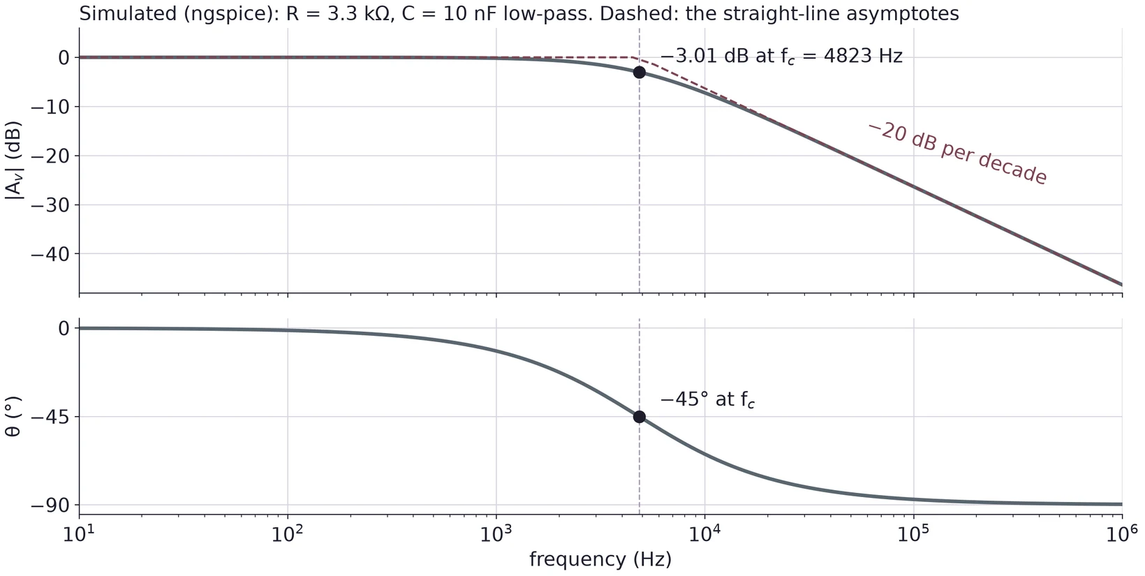
The phase follows the same pattern: near 0° far below , −45° at , and close to −90° far above it. Most of the change happens within a decade on each side of .
| Hz | dB | |||
|---|---|---|---|---|
| 241.1 | 0.9988 | −0.01 | −2.86° | |
| 1607.6 | 0.9487 | −0.46 | −18.43° | |
| 4822.9 | 0.7071 | −3.01 | −45.00° | |
| 14 469 | 0.3162 | −10.00 | −71.57° | |
| 96 458 | 0.0499 | −26.03 | −87.14° |
Between and the gain falls 16.03 dB over a factor of 6.67, which is log10 6.67 = 0.82 of a decade: 19.5 dB per decade, close to the asymptote's 20.
(a) A low-pass uses 10 kΩ and 1 nF. Find , and find , and at 40 kHz.
(b) A low-pass has a gain of −12 dB at 25 kHz. What is its ?
(c) Why must Equation (13) use and not ? Show what goes wrong at .
6 The RC High-Pass Filter and Design
6.1 Swap R and C
Exchange the two parts: the capacitor in series, the resistor to ground, and the output across the resistor. Now the capacitor blocks low frequencies and passes high ones. This is a high-pass filter.
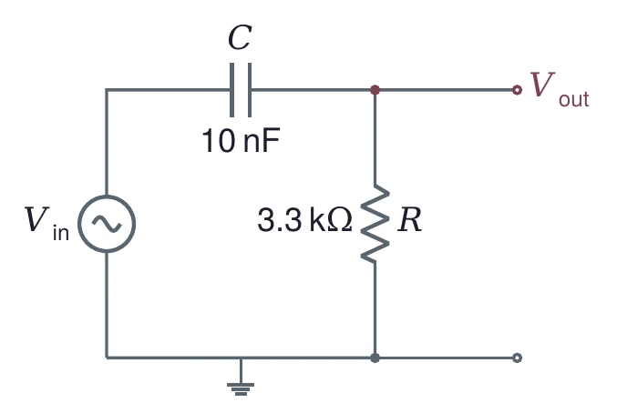
The divider rule gives
with the same . In polar form,
The output leads the input. The lead is close to +90° far below , +45° at , and falls toward 0° far above it. At the gain is again 0.7071, or −3.01 dB.
6.2 Designing for a cutoff
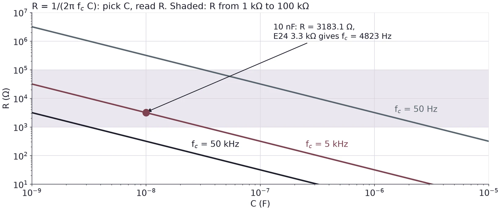
A design starts from the cutoff you want. Equation (14) has two unknowns, so choose one part and compute the other. Choose the capacitor first, because capacitors come in fewer values than resistors. Then compute , round it to a standard value, and recompute with the value you will use.
Keep between about 1 kΩ and 100 kΩ. Much below 1 kΩ, the filter draws enough current that the generator's 50 Ω output resistance starts to matter (Lecture 01). Much above 100 kΩ, the scope's 1 MΩ input sits in parallel with the output and changes the circuit.
Ω. The nearest E24 value is 3.3 kΩ, which gives Hz, 3.5 % below the target. These are the parts of Figures 18 and 24.
6.3 The two filters on one Bode plot
The same R and C, wired both ways round, give mirror images about . The high-pass at has the same gain as the low-pass at , and the same phase with the opposite sign. Below , the high-pass gain rises at +20 dB per decade.
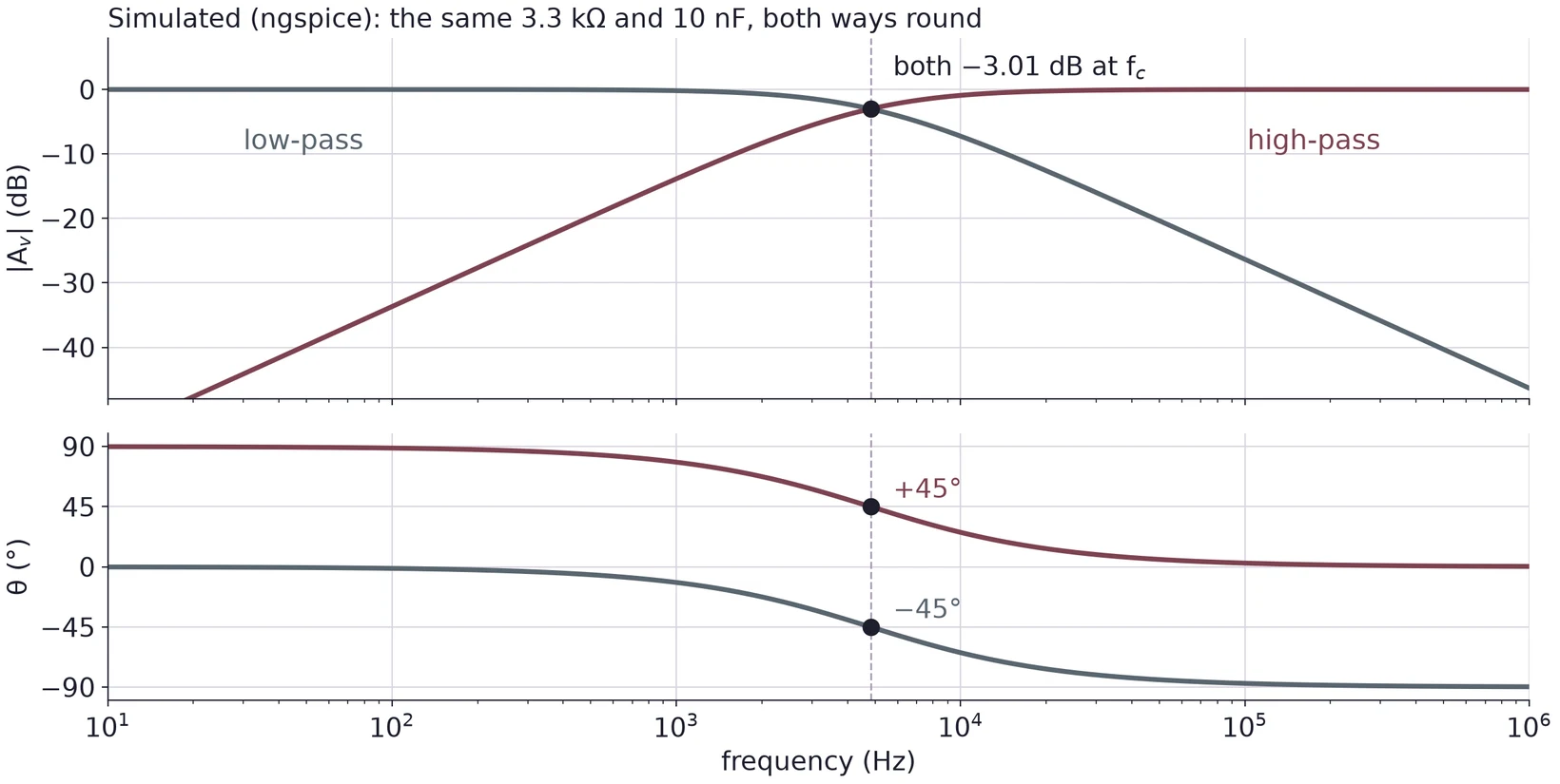
At : 0.0499 at +87.14°. At : 0.3162 at +71.57°. At : 0.9487 at +18.43°. At : 0.9988 at +2.86°. Compare the low-pass table in §5.6.
6.4 Driving a high-pass far below its cutoff
. Equation (20) gives , or dB, and .
The output is mV peak to peak, or 31.04 mV peak. One period at 300 Hz is 3.333 ms, so the output leads by ms. An ngspice transient run of the same circuit gives 62.08 mVpp.
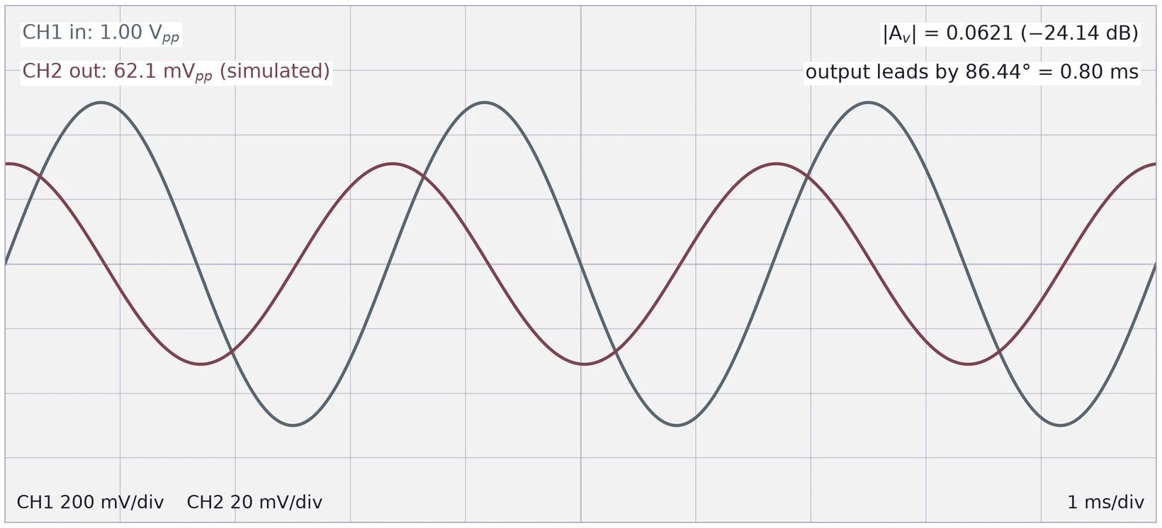
Far below its cutoff, a high-pass makes a small output that is nearly 90° ahead. The output is small, so set the CH2 scale to fit it and say which scale you used.
(a) Design a high-pass for 20 kHz with a 1 nF capacitor. Choose an E24 resistor and recompute .
(b) A high-pass with = 8 kHz is driven at 12 kHz with 1.0 Vpp. Find the output amplitude and the phase.
(c) A classmate builds a high-pass from 220 Ω and 1 µF. What could go wrong when the generator drives it?
7 Measuring a Filter on the Scope
7.1 CH1 on the input, CH2 on the output
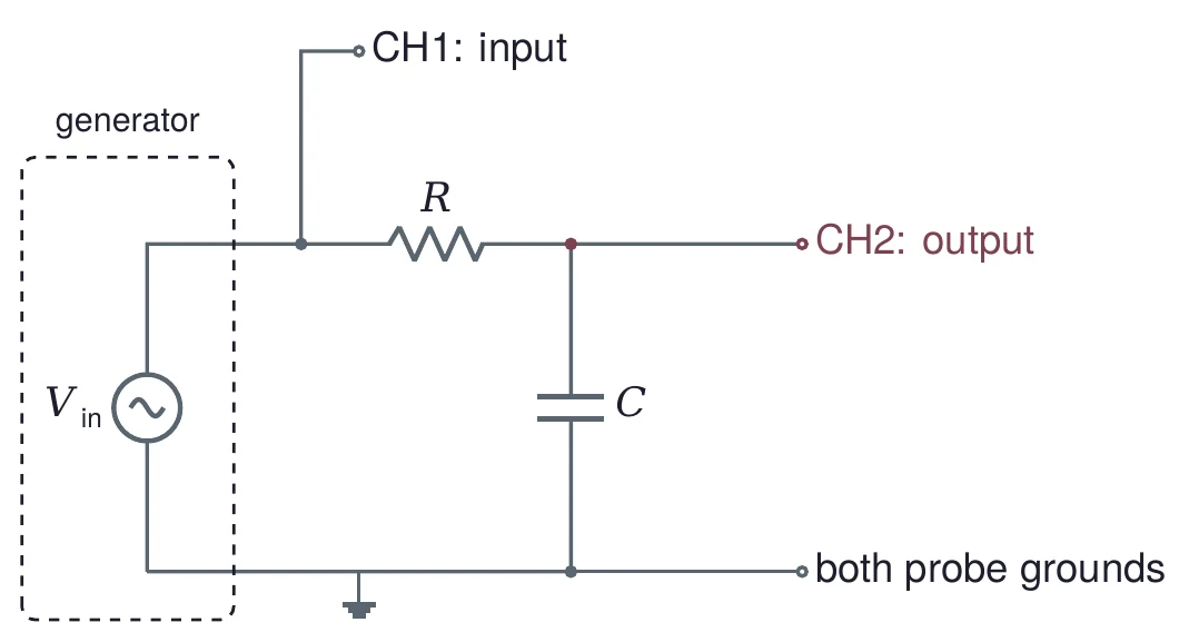
To measure a filter, watch both ends at once. Connect CH1 to the input node and CH2 to the output node, and clip both probe grounds to the circuit ground. Trigger on CH1, the input, so the time axis stays fixed while you compare the two traces. Read both amplitudes at every frequency.
7.2 Finding the cutoff
At the cutoff, . Set the generator near your calculated , then change the frequency until the ratio of the two amplitudes is 0.707. Use the ratio, not alone. The filter's input impedance changes with frequency, so the generator's 50 Ω output resistance (Lecture 01) lets shift a little as you sweep.
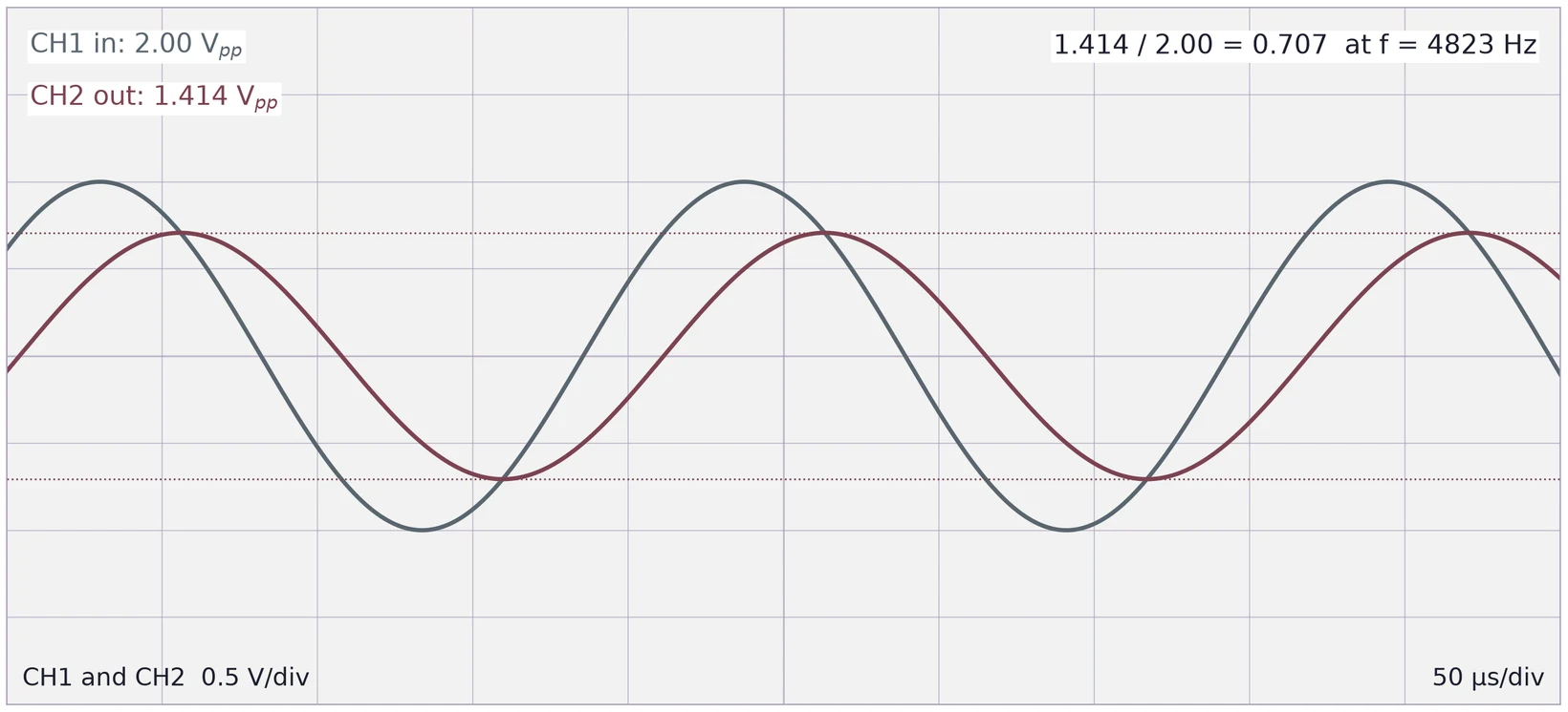
Near the ratio changes slowly with frequency (§8 works out how slowly), so read the amplitudes as precisely as the scope allows: use the scope's amplitude measurements or the cursors, and spread each trace over most of the screen.
7.3 Phase from the time shift
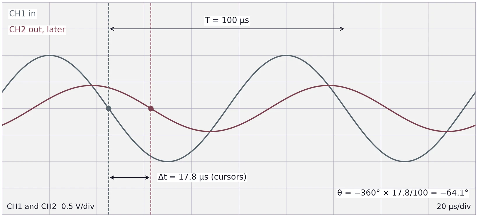
The scope shows time, not phase, so measure the time shift between matching points of the two traces, such as their zero crossings going down. Equation (4) turns it into a phase:
The minus sign is for an output that comes later (a lag). For a high-pass the output comes earlier, and the phase is positive.
Theory gives (§5.4). At 10 kHz, = 100 µs, so the expected delay is µs. Suppose the cursors read = 17.8 µs: . At the cutoff of the same filter, = 207.35 µs and the −45° lag is a delay of = 25.92 µs.
7.4 From measurements to a Bode plot
For each frequency, record , and (and if you want the phase). Compute and plot it against on a log axis. Draw the theory curve for your calculated on the same axes, and mark which points are measured.
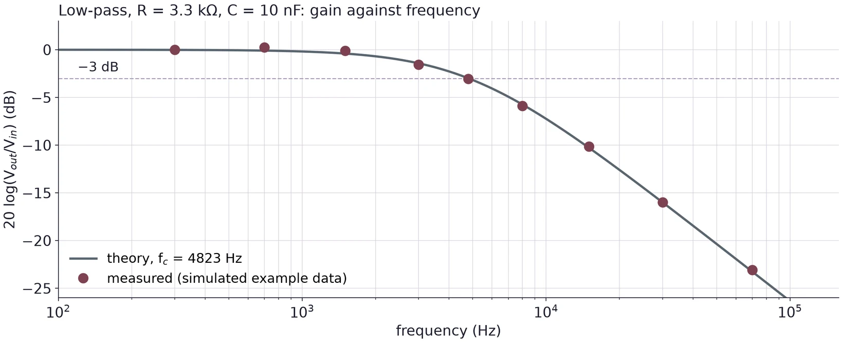
Spread the frequencies evenly on the log axis, and put more of them near , where the curve bends.
(a) A low-pass is driven at 2 kHz, and its output crosses zero 40 µs after the input. Find , then use to estimate .
(b) At one frequency the scope reads 2.04 Vpp on CH1 and 1.40 Vpp on CH2. For a low-pass, is that frequency above or below ?
(c) Why trigger on CH1 rather than CH2 when you measure a phase?
8 Error Analysis
Every task in this course needs an error analysis. For each value you report, state its uncertainty, name the main sources of error, and compare it with the value you expected, simulated or took from a datasheet.
| Measurement | Main error sources |
|---|---|
| Capacitance | The DMM's capacitance accuracy for the range; the leads' own capacitance for small values; a part not fully discharged |
| Calculated or | Tolerance of R and C; use measured values where you have them |
| Measured | Reading the two amplitudes; the slow change of the ratio near ; the generator's frequency display |
| Phase | Reading (cursor placement, trace thickness, noise); the period |
| Bode points | Amplitude readings at small outputs; probe and channel settings; the scope's input loading the output |
8.1 How part tolerance moves the cutoff
Since , the relative errors of R and C carry straight into . If the errors are independent, add them in quadrature. For the worst case, push both the same way.
In quadrature: , so = 4823 Hz ± 11.18 %.
Worst case: both low gives Hz (+16.96 %); both high gives Hz (−13.42 %). The range is not symmetric because goes as .
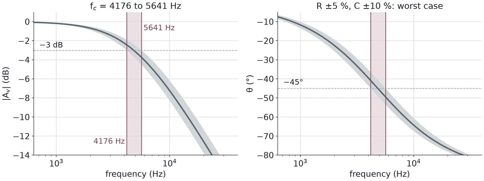
Measure R and C before you build, and calculate from the measured values. Then the comparison with your measured tests the circuit, not the tolerance band.
8.2 How reading errors move the cutoff
Near both curves are fairly flat, so a small reading error becomes a larger frequency error. With , the slope of the magnitude at is . An error of 1 % in (0.00707) is then an error of in : 2.0 % in . The phase has slope rad = −28.65° per unit of at , so a 1° error in phase is a error in : 3.5 % in .
A difference between measured and expected is only meaningful when it is larger than the uncertainty. When it is, say which source most likely explains it, and check that the size fits.