1 Where Lab 5 Sits
Lab 5 is your first transistor lab. First you find the three leads of an NPN and a PNP transistor with the digital multimeter (DMM). Then you bias an NPN transistor with a voltage divider, measure its voltages and currents, and check that it sits in its active region. Last, you warm it with a fingertip and watch the operating point move.
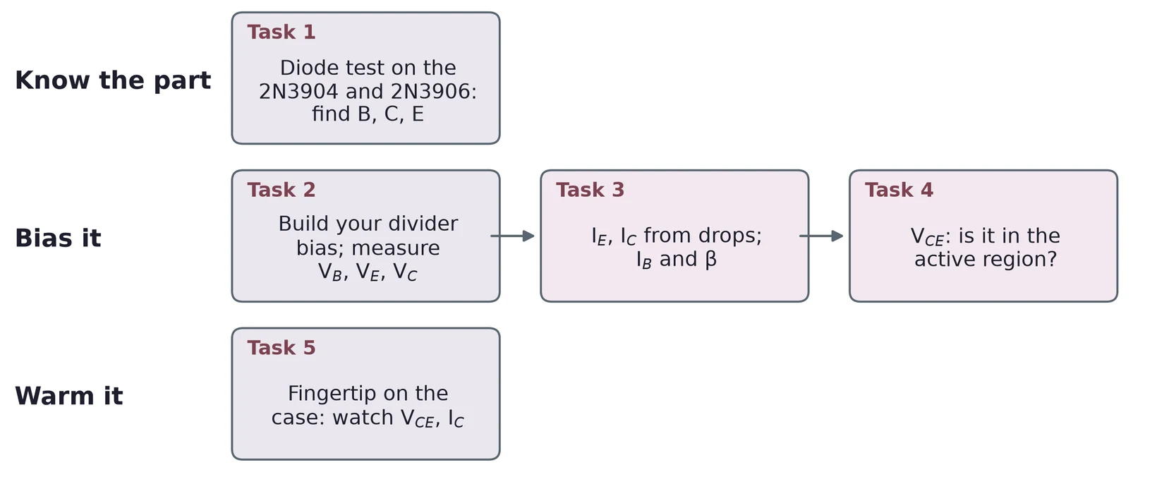
1.1 Task map
| Lab 5 task | What you do | Concept & section |
|---|---|---|
| 1 | Diode-test every lead pair of a 2N3904 and a 2N3906 | Inside the BJT (§2), the DMM test (§3) |
| 2 | Build your divider-bias design at 12 V; measure , , | Notation (§5), divider bias (§7) |
| 3 | Find and from voltage drops, then and | Current gain (§4), measuring (§8) |
| 4 | Find ; check the active region; compare with your targets | Output curves and regions (§6), the load line (§7.6) |
| 5 | Warm the transistor; find a temperature coefficient | Temperature (§9) |
Every task needs an error analysis. Section 10 collects the main error sources, and §8 shows the one trap in this lab that can swamp all the others.
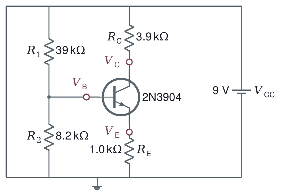
All the worked examples use one teaching circuit: a 2N3904 with = 9 V, = 39 kΩ, = 8.2 kΩ, = 3.9 kΩ and = 1.0 kΩ. Your lab circuit is your own design at 12 V, so your numbers will differ. Lecture 06 builds an amplifier on this same 9 V circuit.
2 Inside the BJT
2.1 Three layers, two junctions
A bipolar junction transistor (BJT) is a sandwich of three doped silicon layers. In an NPN transistor, a thin P-type layer, the base (B), sits between two N-type layers, the emitter (E) and the collector (C). Each boundary is a PN junction, like the diode of Lecture 04: the base-emitter (BE) junction and the base-collector (BC) junction. Each one, forward biased, drops about 0.7 V.
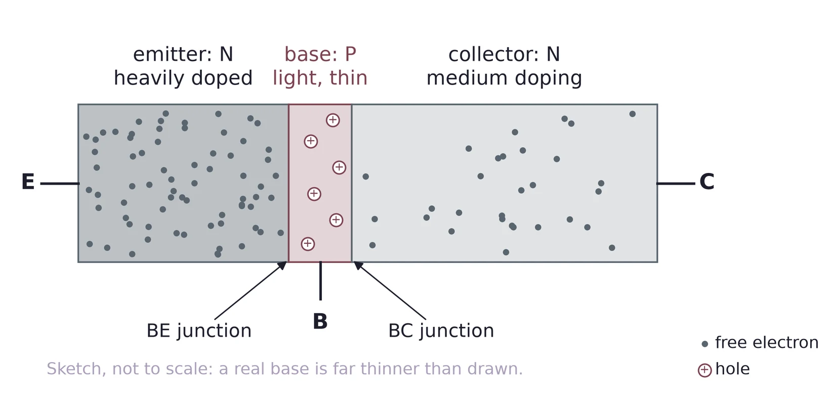
The three layers are not alike. The emitter is heavily doped, so it has many free electrons to send. The base is lightly doped and thin. The collector is moderately doped and the largest, because it has to carry the current away and get rid of the heat. A PNP transistor swaps every type: a thin N-type base between a P-type emitter and collector.
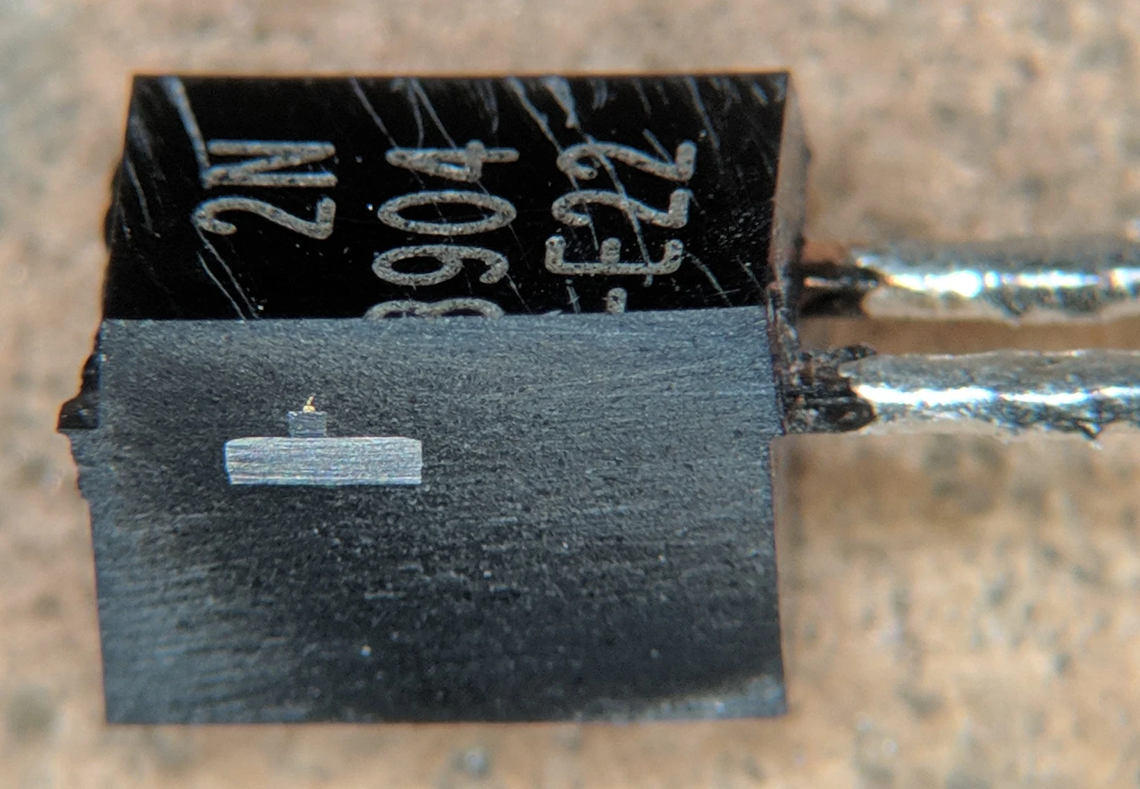

The whole transistor is the small die in Figure 3. The black plastic around it only holds the leads and protects the chip.
2.2 Symbols and the package
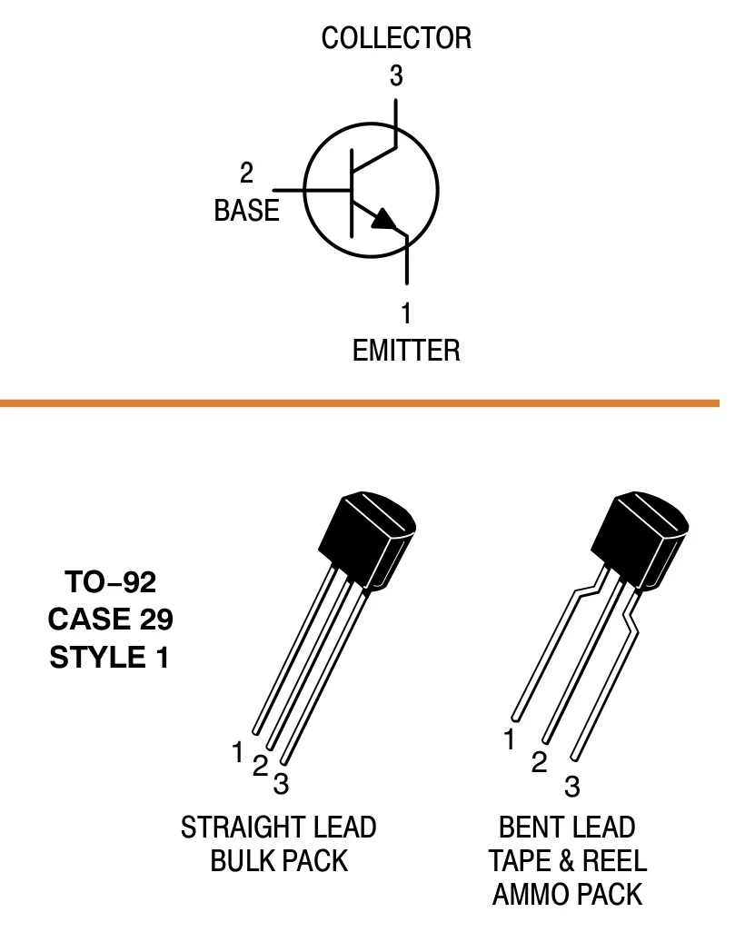
In the circuit symbol, the arrow sits on the emitter. It points the way conventional current flows through the BE junction: out of the emitter in an NPN, into the emitter in a PNP. A memory aid: the NPN arrow is "Not Pointing iN".
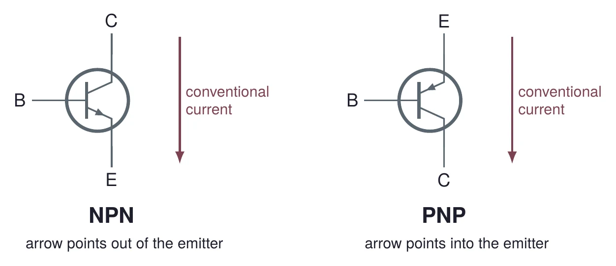
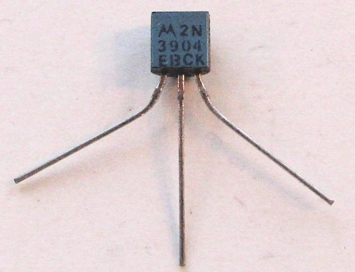
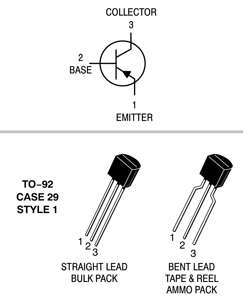
The 2N3904 (NPN) and its partner the 2N3906 (PNP) are small-signal transistors in a TO-92 plastic package. Hold the flat face toward you with the leads down, and the leads are emitter, base, collector from left to right. The datasheet numbers them pins 1, 2 and 3. Other parts in the same package can use another order, so always check the datasheet of the exact part.

2.3 How the current gets across
In normal use, the BE junction is forward biased and the BC junction is reverse biased. The forward-biased BE junction lets the emitter push a large flow of electrons into the base. If the base were thick, these electrons would meet holes there and recombine, and they would all come out through the base lead. But the base is thin and has few holes. Most electrons cross it before they recombine. When they reach the BC junction, its electric field (the same field that blocks current in a reverse-biased diode) sweeps them into the collector.
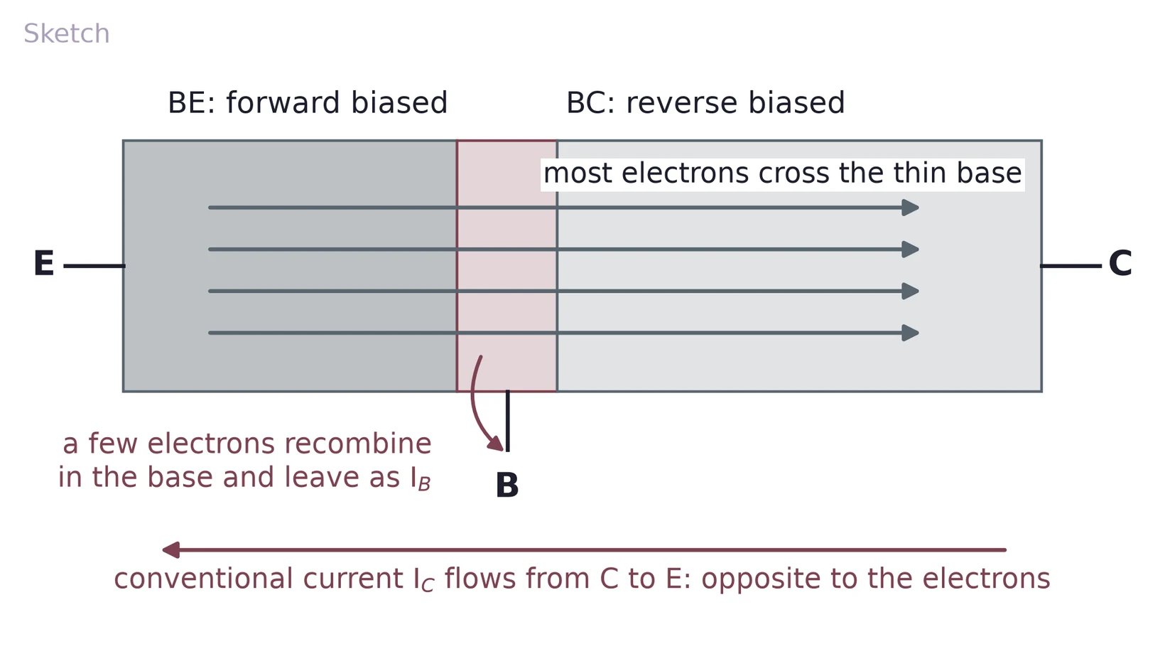
So a small base current controls a much larger collector current. Electrons travel from emitter to collector, while conventional current, which is defined for positive charge, flows from collector to emitter. Keep the two apart when you read a sketch with electrons on it.
2.4 Three currents, one node
Treat the transistor as one node. Current flows in at the base and the collector and out at the emitter, so Kirchhoff's current law gives
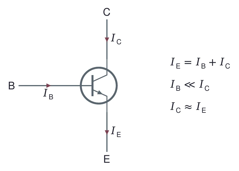
Because only a few electrons recombine in the base, is much smaller than , usually by a factor of 100 or more. For many design steps you can then take .
(a) In a PNP transistor, which way does conventional current flow through the emitter lead? Which carriers cross the base?
(b) An NPN has = 3.6 mA and = 3.624 mA. Find .
(c) Why must the base be thin? What would happen to and if it were as thick as the collector?
3 Checking a Transistor with the DMM
3.1 Two diodes back to back
To a DMM, a BJT looks like two diodes that share the base. In an NPN, the P-type base is the anode of both: one diode points from the base to the collector, the other from the base to the emitter. In a PNP, the N-type base is the cathode of both, so both diodes point into the base.
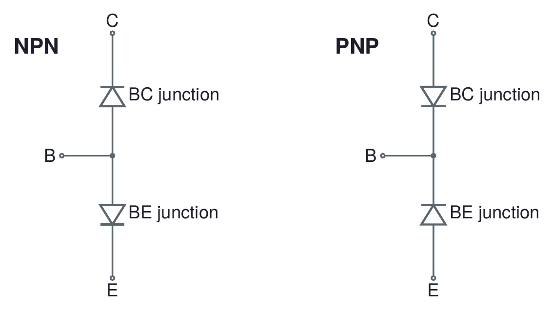
This model is only good for a meter check. Two separate diodes wired this way do not make a transistor, because they have no thin shared base for the electrons to cross.
3.2 Diode-test mode
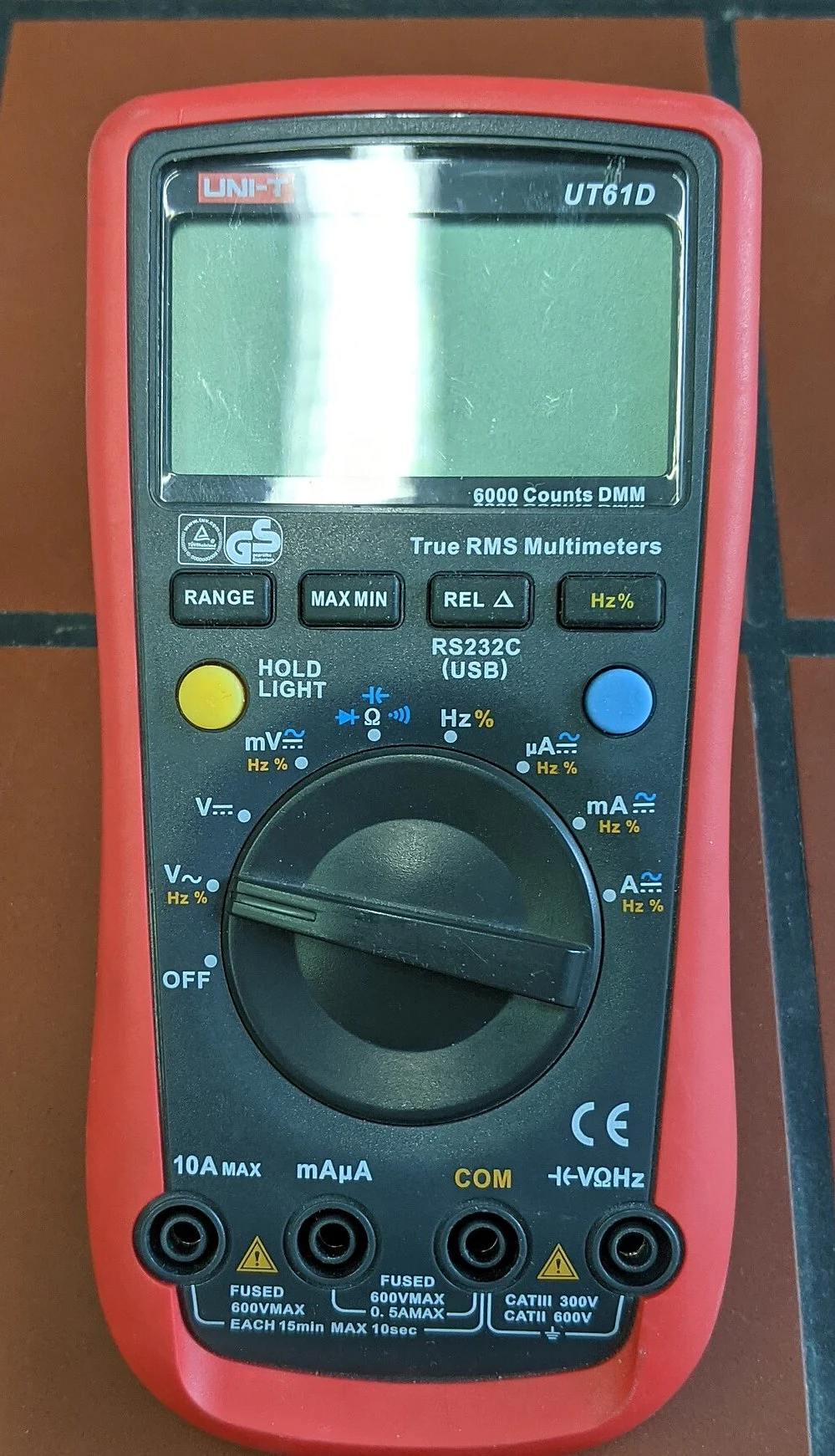
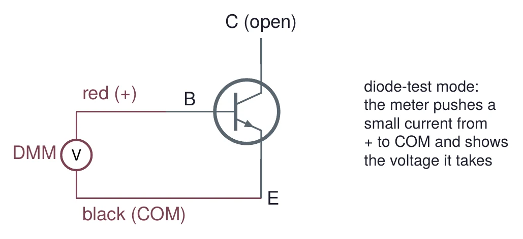
In diode-test mode, the DMM pushes a small, fixed current out of its red (+) lead and into its black (COM) lead, and shows the voltage that takes. A forward-biased silicon junction shows its junction voltage, a few tenths of a volt. A reverse-biased junction, or two leads with no junction between them, shows OL (over limit).

3.3 Finding the base and the type
Test all six ordered pairs of leads. For an NPN, the pattern is:
| Red (+) | Black (COM) | An NPN reads |
|---|---|---|
| B | C | a junction voltage (BC forward) |
| B | E | a junction voltage (BE forward) |
| C | B | OL |
| E | B | OL |
| C | E | OL |
| E | C | OL |
Only two of the six pairs conduct, and they share one lead: the base. If the shared lead is on the red probe, the part is an NPN. Before you test the 2N3906, use Figure 9 to predict its pattern. The two junction voltages usually differ a little, which hints at which lead is the emitter; the datasheet pinout confirms it.
A shorted transistor reads near 0 V on some pair in both directions; an open one reads OL on a pair that should conduct. Both are worth recording, since a damaged part explains a circuit that will not bias.
(a) You test an unknown transistor. Red on lead 2 and black on lead 1 reads a junction voltage; red on lead 2 and black on lead 3 also does. Every other pair reads OL. Which lead is the base, and is it NPN or PNP?
(b) Write the six-row pattern you expect for a PNP before you measure it.
(c) Why does the pair C to E read OL in both directions, even though it passes through two junctions?
4 Current Gain and the Datasheet
4.1 DC current gain
The ratio of collector current to base current is the DC current gain, :
Datasheets call it . The ratio of collector current to emitter current is , which is a little below 1.
A transistor has = 2.4 mA and = 12 µA. Then = 2.4 mA / 12 µA = 200, = 2.4 mA + 0.012 mA = 2.412 mA, and = 2.4/2.412 = 0.9950.
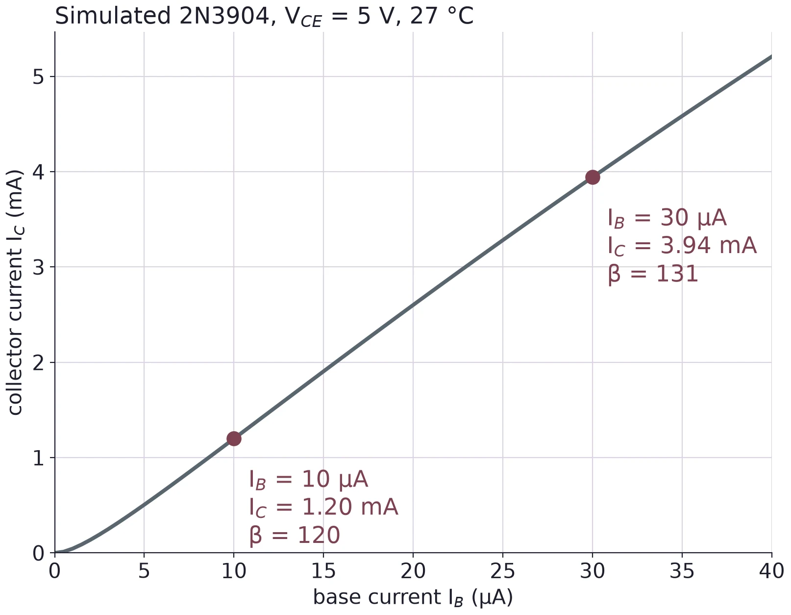
Figure 13 shows that β is not one fixed number. The curve is close to a straight line, but its slope from the origin changes with the current. The model is one typical part; your transistor will differ.
4.2 What the datasheet promises
The datasheet table gives at several collector currents, with a minimum and sometimes a maximum. For the 2N3904 at 1 mA it guarantees only that β is at least 70. At 10 mA, β lies between 100 and 300. The same table gives the collector-emitter breakdown voltage = 40 V: never put more than that across collector and emitter.
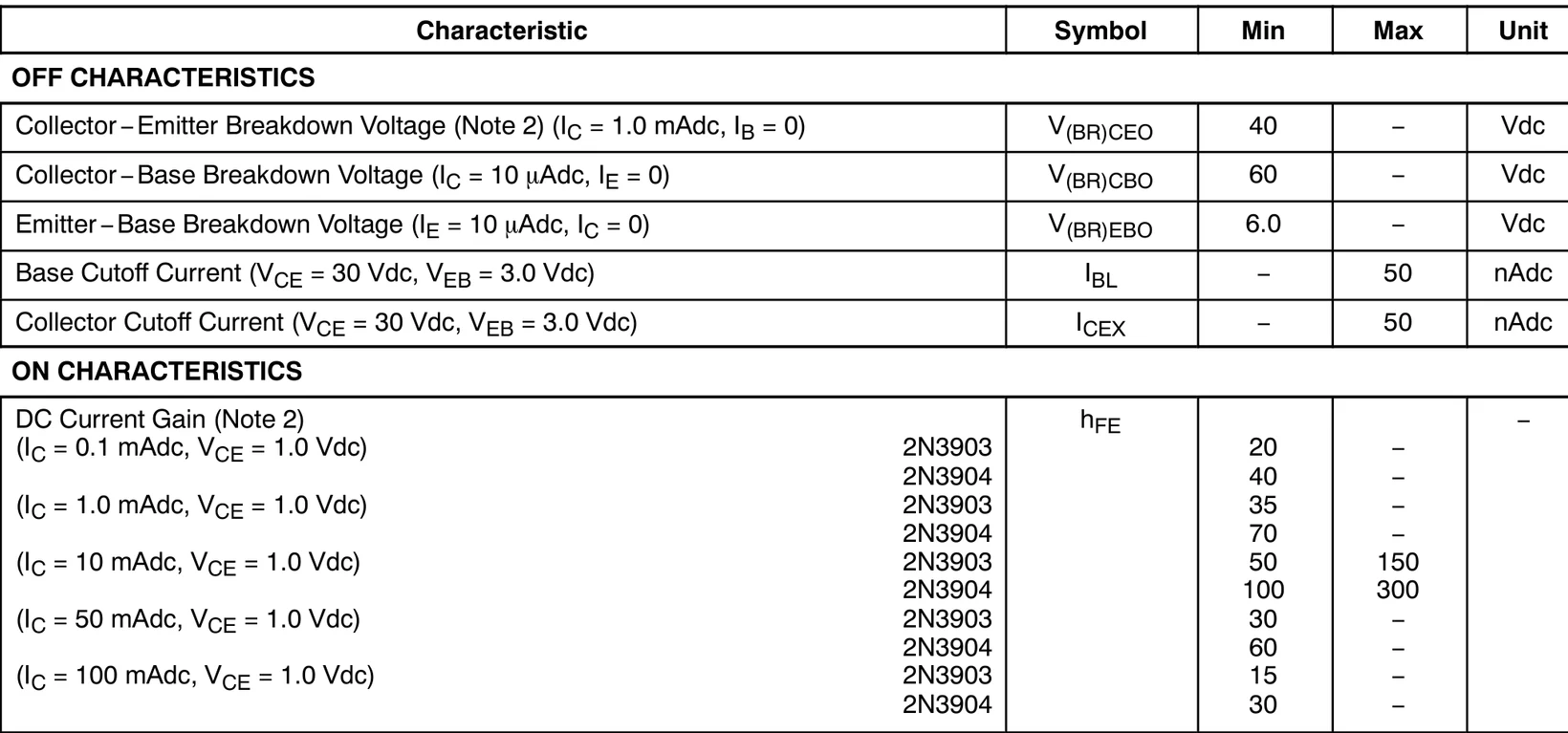
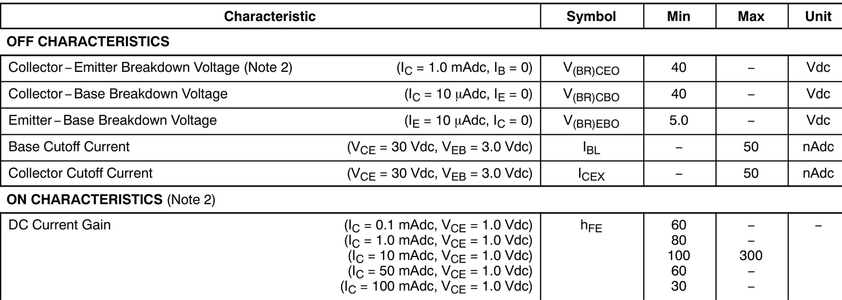
A design must work for any part the datasheet allows, so it uses the minimum β at the planned current. In Task 3 you compare your measured β with this table: check that you read the row for your collector current.
4.3 β changes with current and temperature
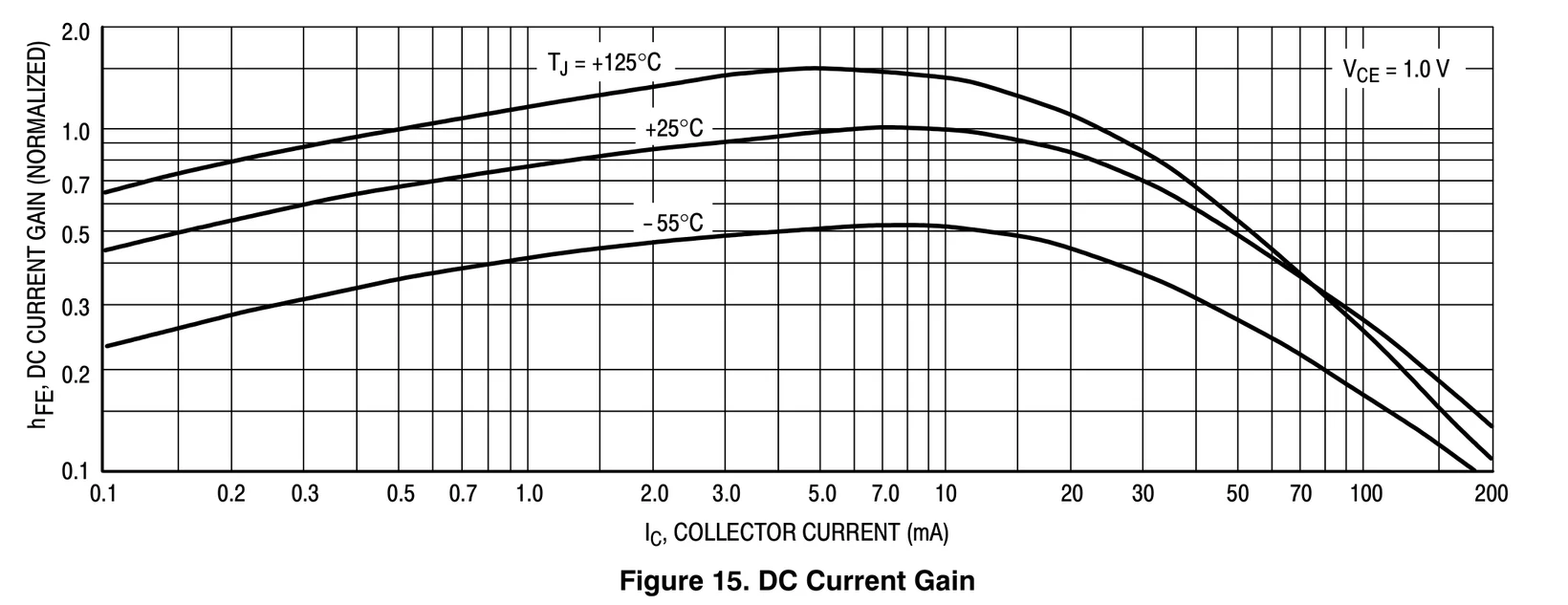
Figure 16 shows how of a typical 2N3904 changes. It is normalized: the 25 °C curve peaks at 1.0, near 5 to 10 mA. Gain falls at low current, falls faster above about 20 mA, and rises with temperature at most currents.
As a rough guide, small-signal transistors (low-power parts like the 2N3904) have β of about 100 to 300, and power transistors about 20 to 100. "Small-signal" here names the kind of part, made for small currents and powers; it is not the size of the signal you feed it.
(a) A transistor has = 5.0 mA and = 125. Find , and .
(b) Use Figure 14 to give the range of β a 2N3904 may have at 10 mA. If = 50 µA, what range of follows?
(c) From Figure 16, about how much does the gain change from 25 °C to 125 °C at 1 mA?
5 Notation and Base Bias
5.1 Double and single subscripts
Transistor circuits use one naming scheme. Upper-case letters mean DC values. A double subscript with a repeated letter is a supply: for the collector supply, for the base supply, for the emitter supply. A double subscript with two different letters is the voltage between two terminals: from base to emitter, from collector to emitter. A single subscript is a node voltage measured to ground: , , .
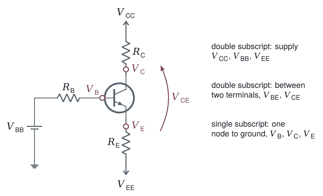
So you measure , and with the black lead on ground, and compute and from them.
5.2 Three ways to connect it
A transistor has three leads, and a signal needs an input and an output, so one lead is shared. The connection is named for that shared lead. In the common-emitter (CE) circuit the input goes to the base and the output comes from the collector. In the common-collector (CC) circuit, also called the emitter follower, the output comes from the emitter. In the common-base (CB) circuit the input goes to the emitter.
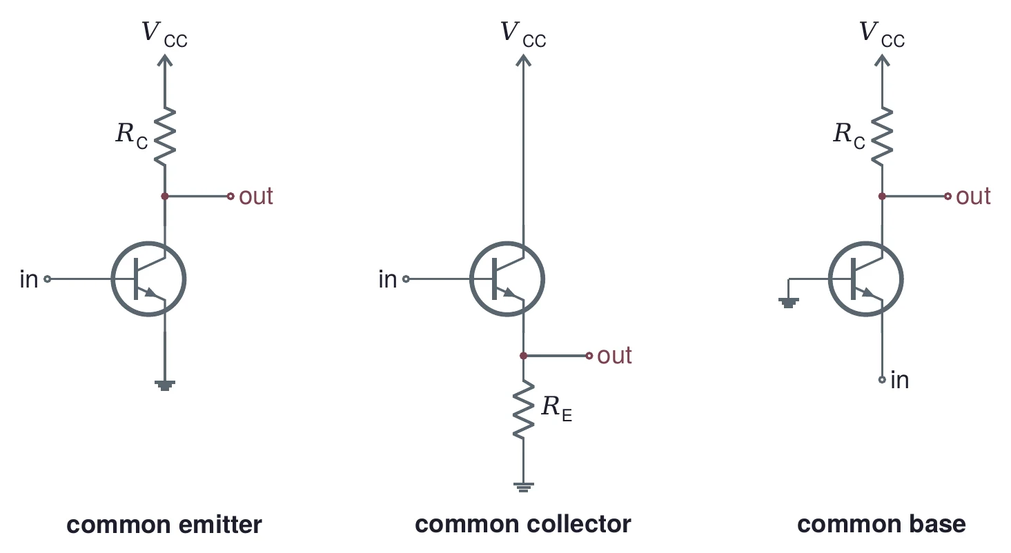
This lab sets the DC operating point of a common-emitter stage. Lecture 06 adds the signal and turns it into an amplifier.
5.3 Base bias, step by step
Biasing means choosing DC voltages and currents that put the transistor where you want it. The simplest way is base bias: one resistor from a supply into the base.
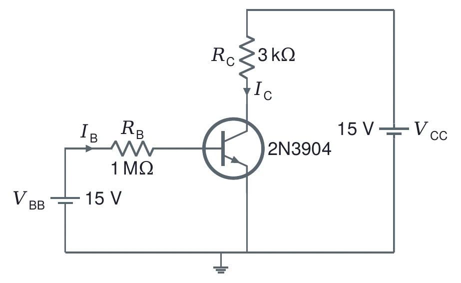
Work from the base to the collector. The emitter is grounded, so = 0 and = 0.7 V. Ohm's law across gives the base current; β gives the collector current; the drop across gives the collector voltage:
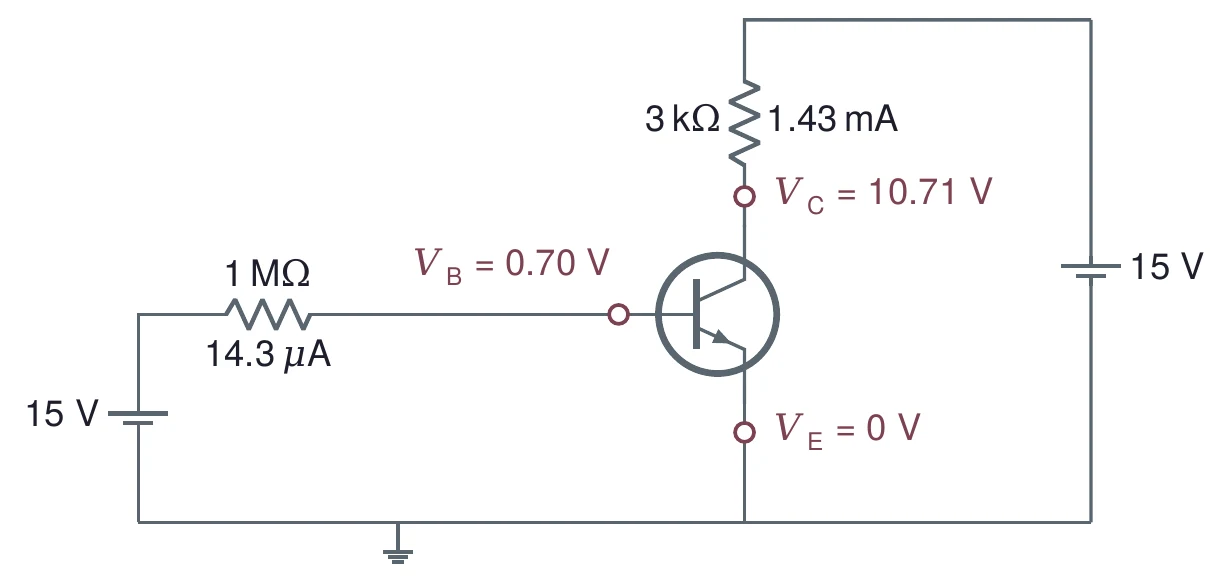
= (15 − 0.7) V / 1 MΩ = 14.30 µA. = 100 × 14.30 µA = 1.430 mA, and = 1.430 + 0.0143 = 1.444 mA. = 15 − 1.430 mA × 3 kΩ = 15 − 4.29 = 10.71 V. With the emitter grounded, = 10.71 V.
5.4 VCE tells you where it sits
= 10.71 V is well above 0.2 V and below the 15 V supply, so the transistor is in its active region (§6), where holds. That is the check you make in Task 4.
5.5 Base bias depends on β
The trouble with base bias is that β sets directly. Run the same numbers with other values of β:
| β | ||
|---|---|---|
| 100 | 1.430 mA | 10.71 V |
| 200 | 2.860 mA | 6.42 V |
| 300 | 4.290 mA | 2.13 V |
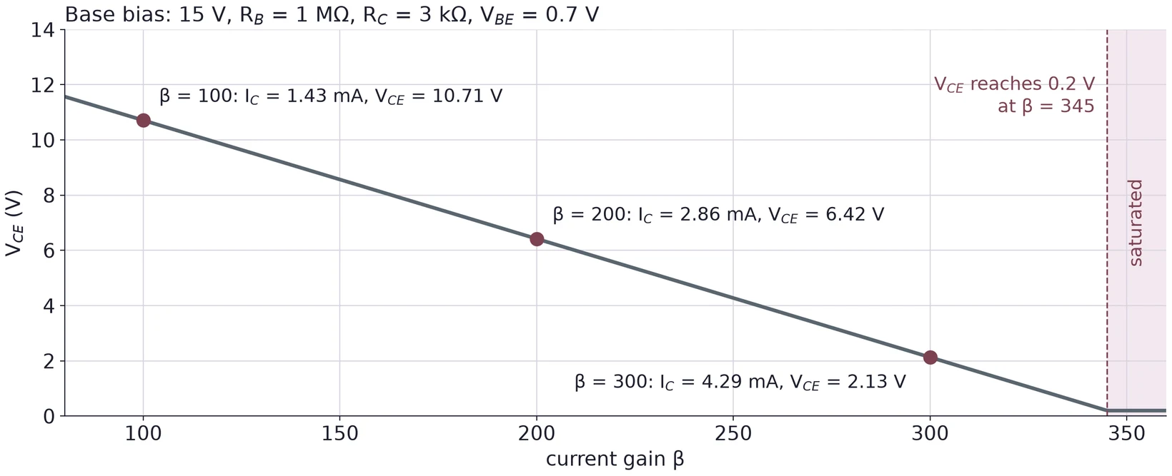
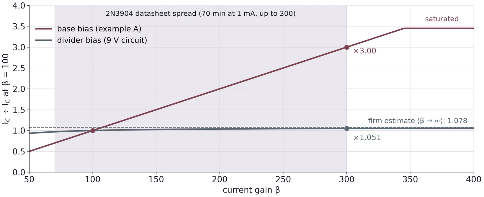
The collector current cannot exceed what lets through with the transistor fully on: 15 V / 3 kΩ = 5.0 mA. falls to 0.2 V when = (15 − 0.2)/3 kΩ = 4.93 mA, which takes β = 345. Since two 2N3904s from one bag can differ by a factor of two or three in β, a base-bias circuit built for one part may saturate with the next. Base bias is fine for a switch, which is meant to saturate. For an amplifier, use divider bias (§7).
(a) A base-bias circuit has = 10 V, = 470 kΩ and = 2.2 kΩ. Find , and for β = 150.
(b) For the circuit in (a), what β puts at 0.2 V?
(c) You measure = 0.66 V and = 0.12 V in a base-bias circuit with a grounded emitter. Which region is the transistor in?
6 Output Characteristics and the Three Regions
6.1 Output curves
Hold the base current fixed and sweep , and the collector current traces one output curve. A family of curves, one per , describes the transistor completely. Figure 22 shows a family simulated with the onsemi model.
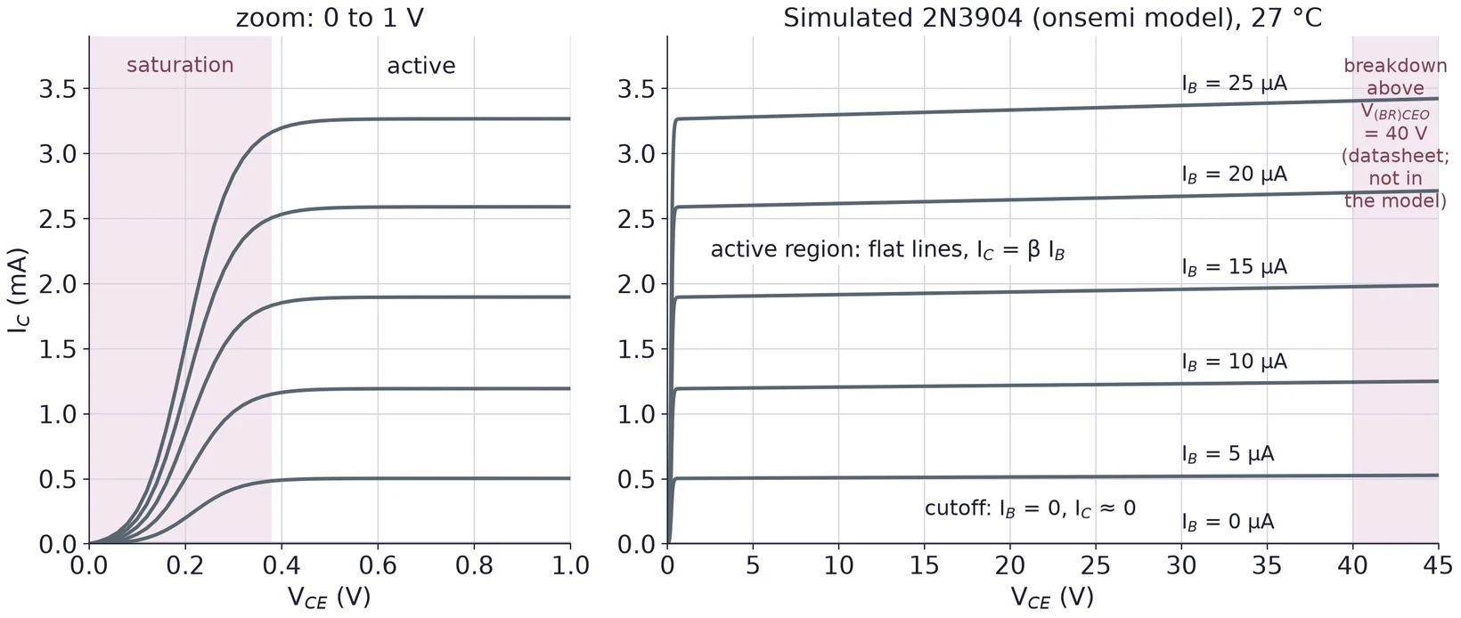
Near = 0 each curve climbs steeply: the collector cannot collect everything the emitter sends yet, because the BC junction is not reverse biased. That steep part is saturation. Above a few tenths of a volt the curves flatten: is set by and hardly by . That flat part is the active region, where . With = 0 almost no current flows: cutoff. Far to the right, at = 40 V, the BC junction breaks down and the current shoots up; the datasheet sets this limit, and the circuit must stay below it.
In a real transistor the flat lines tilt up a little as grows (the Early effect). The onsemi model has almost no tilt, so its lines are nearly flat. In saturation, its curves bend over a range of about 0.3 to 0.4 V; the datasheet below gives the saturation voltage you can count on.
6.2 Saturation: the switch is closed
In saturation the transistor acts like a closed switch with a small voltage across it. The base gets more current than the collector circuit can use: is limited by the resistors, not by β, so . Figure 23 shows how drops as the base current grows, for four fixed collector currents.
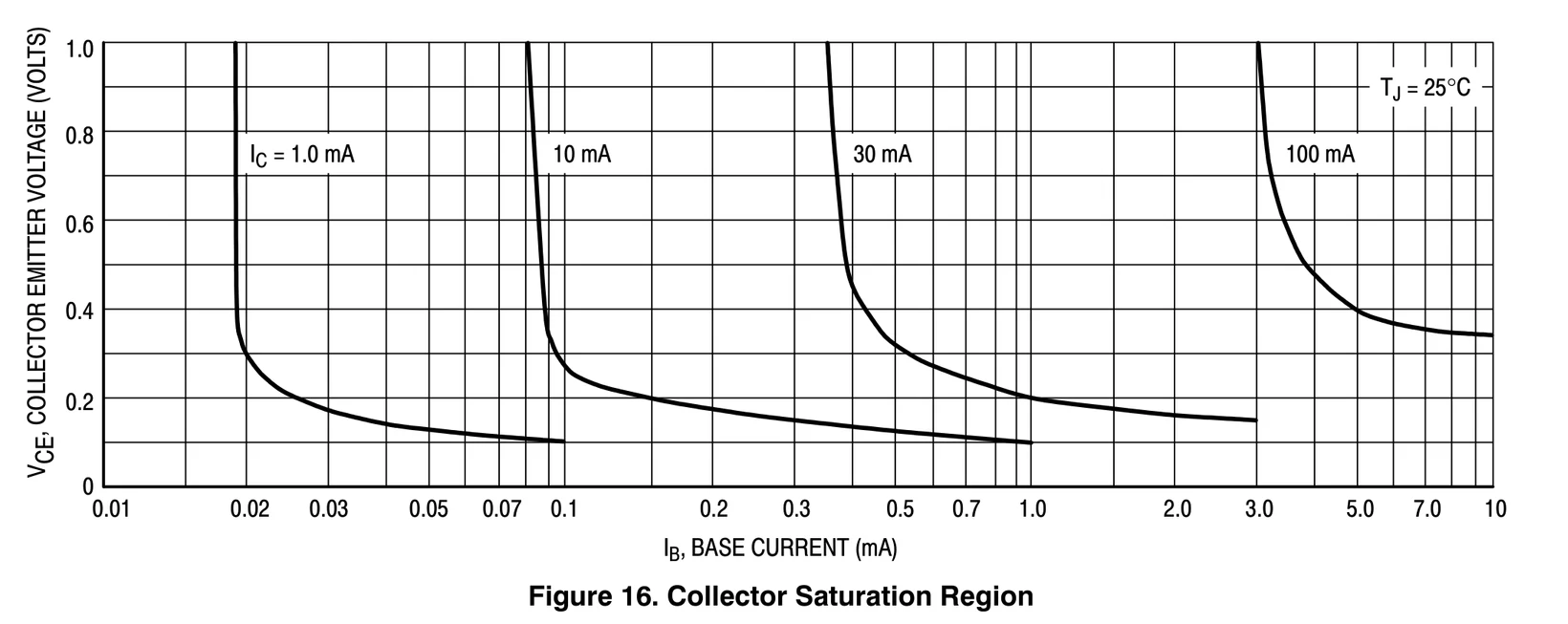
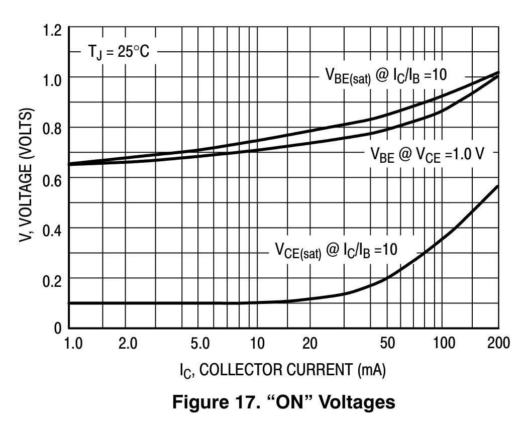
Figure 24 also gives a useful active-region number: at = 1 mA, of a typical 2N3904 is about 0.65 V, a little below the 0.7 V we assume by hand. A few rows below the part of the table in Figure 14, the datasheet guarantees of at most 0.2 V at = 10 mA with = 1 mA.
6.3 Which region?
| Region | BE junction | BC junction | Check from your measurements |
|---|---|---|---|
| Cutoff (switch open) | off: too small to conduct | reverse | ; close to the supply |
| Active (amplifier) | forward, about 0.6 to 0.7 V | reverse | well above 0.2 V and below the supply; |
| Saturation (switch closed) | forward | forward | about 0.2 V or less; below |
The BC junction is reverse biased when the collector is above the base, so is a quick active-region check for an NPN. For Task 4, compute and from your three node voltages and place your transistor in the table.
(a) You measure = 2.35 V, = 1.68 V and = 1.85 V. Find and . Which region?
(b) Why is false in saturation?
(c) Why does a switch circuit want saturation, but an amplifier wants the active region?
7 Voltage Divider Bias
7.1 The divider holds the base voltage
Voltage-divider bias replaces with a divider, and , and adds an emitter resistor . If the base current is small next to the current in the divider, the divider sets the base voltage on its own, as in Lecture 01:
The rest follows in a chain, with no β anywhere:
is what makes this work. If tries to rise, rises with it; since the divider holds , that leaves less , and the transistor turns down again. This is negative feedback, and it is why divider bias barely notices β.
7.2 Seen from the base, the divider is a Thévenin source
Equation (4) ignores the base current. To see when that is fair, replace the divider by its Thévenin equivalent, as in Lecture 01: a source behind a resistance .
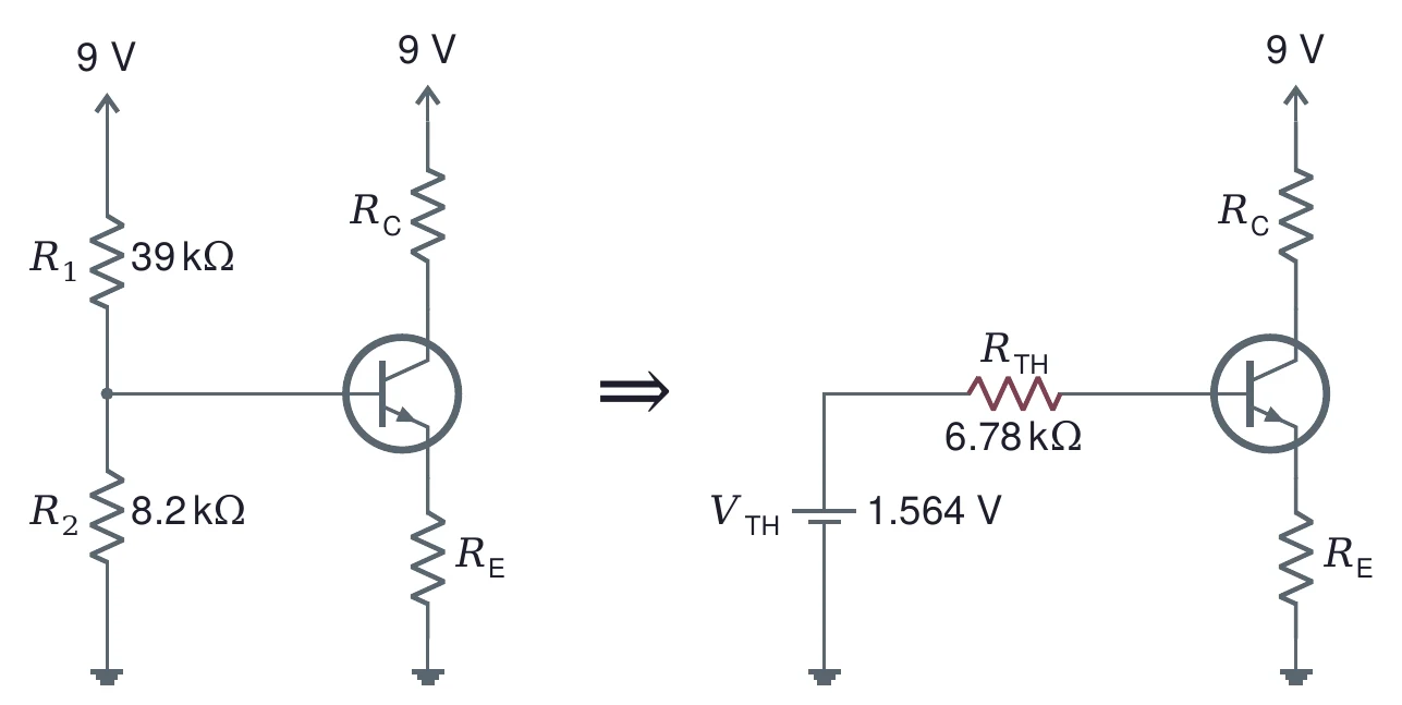
Write Kirchhoff's voltage law from through the base and emitter to ground, with :
Looking into the base, the divider sees a load of : the emitter resistor multiplied up by the transistor. Lecture 01's firm-source rule asks for under a tenth of the load. With β + 1 ≈ β, that gives the firm-divider rule:
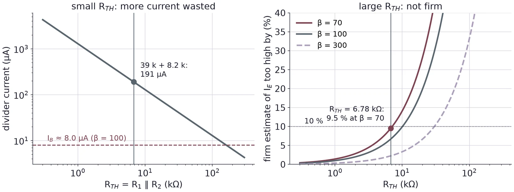
. Then the term in Equation (7) is under a tenth of , and the simple chain of §7.1 is within about 10 % of the exact answer. Use the datasheet's minimum β at your planned current.
The firm rule is the same as asking the divider current to be much larger than the base current. A firm divider passes at least about ten times .
7.3 Design steps 1 to 3: VE, RE, RC
A divider-bias design starts at the emitter and works outward. We design the teaching circuit for = 9 V and a collector current near 1 mA.
Step 1, emitter voltage. A common choice is a tenth of the supply: = 0.1 × 9 V = 0.9 V. A volt or so across makes the uncertain 0.7 V of matter less.
Step 2, emitter resistor. . A round of 1.0 kΩ gives = 0.9 V / 1.0 kΩ = 0.90 mA, close to the 1 mA aim.
Step 3, collector resistor. Put at half the supply, 4.5 V, so the collector has room to swing both ways (Lecture 06). Then = 0.9 + 4.5 = 5.4 V and = (9 − 5.4) V / 0.90 mA = 4.0 kΩ. The nearest E24 value is 3.9 kΩ.
7.4 Steps 4 to 6: pick R1 and R2, then recompute
Step 4, base voltage. = 1.6 V.
Step 5, firm limit. The 2N3904 datasheet promises β ≥ 70 at 1 mA, so < 0.1 × 70 × 1.0 kΩ = 7.0 kΩ.
Step 6, the divider. The divider must give = and = 7.0 kΩ. Since , and in the same way :
Round to E24: 39 kΩ and 8.2 kΩ. Rounding down makes a little smaller, which keeps the divider firm.
Recompute with the real values. = 9 × 8.2/47.2 = 1.564 V and = 6.78 kΩ, under the 7.0 kΩ limit. The firm estimate gives = 1.564 − 0.7 = 0.864 V, = 0.864 mA, = 9 − 0.864 × 3.9 = 5.63 V and = 4.77 V. Equation (7) with β = 100 gives the exact values: = 0.864/(1 + 6.78/101) = 0.809 mA, = 0.801 mA, = 8.0 µA, = 1.509 V, = 0.809 V, = 5.875 V and = 5.07 V.
The firm estimate is 6.7 % above the exact at β = 100 and 9.5 % above at β = 70: that is what "within about 10 %" means. Figure 27 compares the two bias methods over the whole β range. From β = 100 to 300, divider bias changes by 5 %; base bias triples it.
7.5 Too small wastes current, too large is not firm
Only the ratio of to sets ; their size sets . Small resistors make a firm divider but draw a lot of current from the supply and load any signal source you connect later. Large resistors save current but stop being firm, and starts to follow β again. Our divider draws 9 V / 47.2 kΩ = 191 µA, about 24 times the 8.0 µA base current at β = 100.
7.6 The DC load line and the Q point
Whatever the transistor does, Kirchhoff's voltage law around the collector loop must hold. With :
On the output-curve axes this is a straight line, the DC load line. Its ends are the two extremes. Fully on ( = 0), = 9 V / 4.9 kΩ = 1.84 mA. Fully off ( = 0), = 9 V. The bias picks one point on the line, the quiescent or Q point. Ours sits near the middle, which Lecture 06 needs for an amplifier.
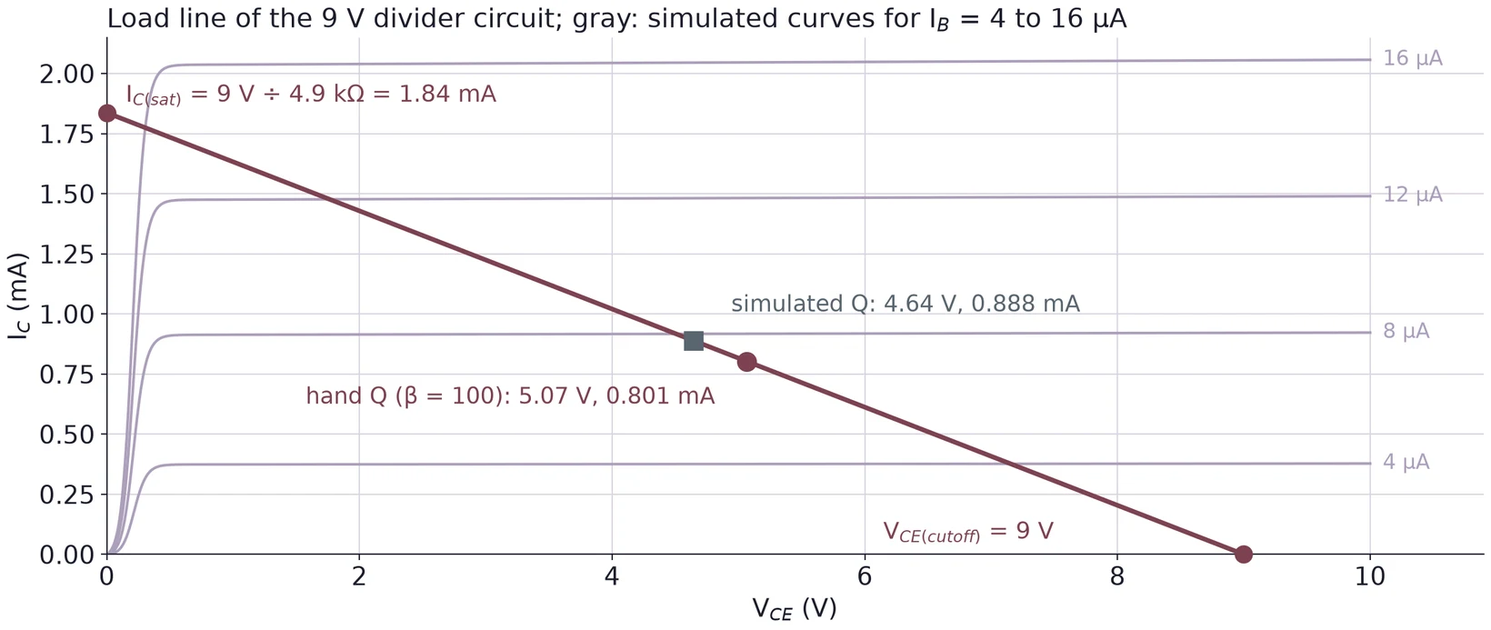
At the Q point the transistor dissipates = 5.07 V × 0.801 mA = 4.1 mW, far below the 625 mW the 2N3904 datasheet allows at 25 °C.
(a) Design a divider-bias circuit for = 10 V and ≈ 2 mA, with = 0.1 and = /2. Find and , then .
(b) Use the minimum β of 70 for the firm rule in (a). Find the largest allowed , then and ; round to E24 values and recompute and .
(c) Find and of your design in (b) with Equation (7) for β = 70 and β = 300. Draw its load line and mark both Q points.
8 Measuring the Operating Point
8.1 Currents from voltage drops
Breaking a circuit to put a DMM in series is slow and changes the circuit. In this lab you find the emitter and collector currents from the voltage across a known resistor instead:
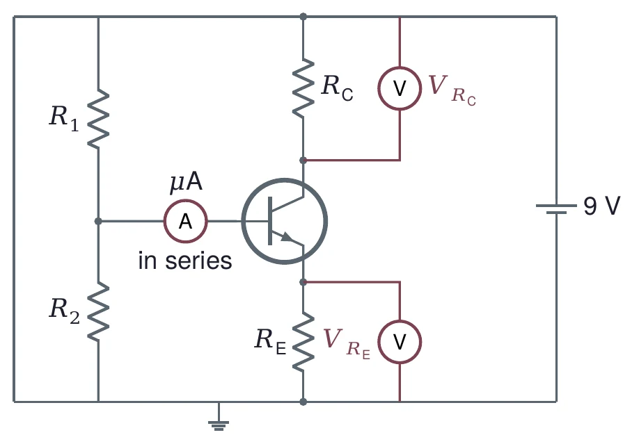
Measure each resistor out of the circuit first (Task 2) and use the measured value, not the color code. equals , since goes to ground. is ; you can measure it directly across or subtract two node voltages, but the direct reading is better (§10).
8.2 IB from a difference is a trap
Equation (1) says . The trouble is that and differ by about 1 %, while each carries an uncertainty of about 1 % too. When you subtract two nearly equal numbers, their absolute errors add (in quadrature) and the difference is small, so its relative error is huge.
Suppose = 1.010 mA and = 1.000 mA, each known to ±1 %. Then = 10 µA, with
So = 10 ± 14.2 µA (±142 %): the result cannot even tell you the sign. At ±0.5 % each, it is still ±7.1 µA (±71 %), and β from it is meaningless.
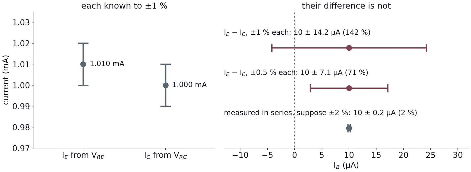
The same trap catches , the difference of the two divider currents: in the teaching circuit, 192.1 µA − 184.0 µA = 8.0 µA. Better ways to get :
- Measure it directly with the DMM's µA range in series with the base, as in Figure 30. The meter's small drop changes a little; remove it before you measure the other voltages.
- If you must subtract, read both drops with the same meter on the same range, so its gain error largely cancels, and state the uncertainty you get.
8.3 Hand calculation, simulation and measurement
A SPICE simulation with the manufacturer's model is a third check, next to your hand calculation and your measurement. Here is the teaching circuit both ways:
| 9 V circuit | Hand: = 0.7 V, β = 100 | ngspice, onsemi model, 27 °C |
|---|---|---|
| 1.509 V | 1.511 V | |
| 0.809 V | 0.895 V | |
| 5.875 V | 5.538 V | |
| 5.066 V | 4.643 V | |
| 0.801 mA | 0.888 mA | |
| 8.01 µA | 7.79 µA | |
| , β | 0.700 V, 100 | 0.615 V, 114.0 |
agrees to 2 mV, because the firm divider holds it. differs by 86 mV, and that comes almost entirely from : the model's 2N3904 drops 0.615 V at this current, not 0.7 V. Put the model's own = 0.615 V and β = 114 into Equation (7) and the hand result matches ngspice to within 1 mV. So when your measured is off from your design, look at first. Both columns place the transistor in the active region: is far above 0.2 V and is above .
(a) In a divider-bias circuit with = 680 Ω and = 2.7 kΩ, you read = 1.093 V and = 4.320 V. Find , , and by subtraction. What does the subtraction suggest about β, and why should you not trust it?
(b) A µA reading in series with the base gives 7.3 µA for the circuit in (a). Find β.
(c) Your measured is 0.10 V above your design value, and matches. What is the most likely reason?
9 Temperature Effects
9.1 VBE falls and β rises as it warms
At a fixed current, the forward voltage of a silicon junction falls by about 2 mV for each degree Celsius it warms. β rises with temperature too (Figure 16). Both changes push up.
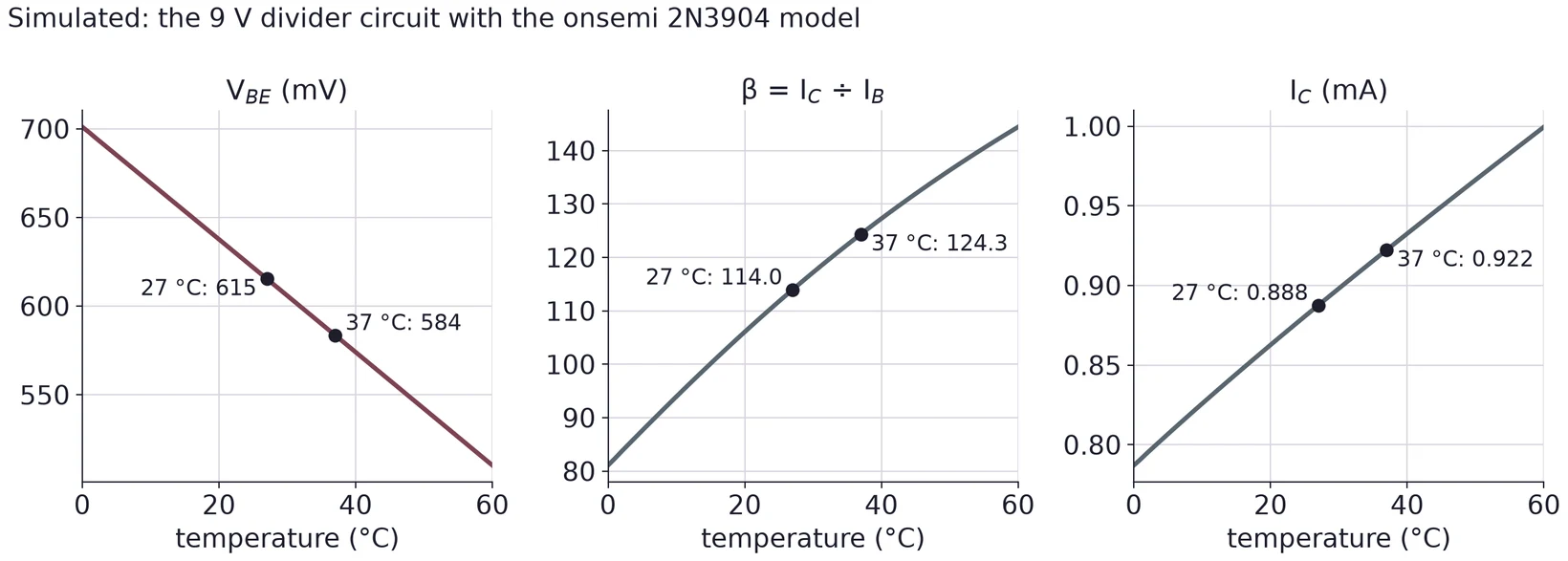
The model's falls 3.2 mV/°C, faster than a typical part. Use the simulation to see which way things move, and your own measurement for the size.
9.2 A temperature coefficient
A temperature coefficient is the change in a quantity per degree. Name the quantity and its units: in mV/°C, or the fractional change of per degree in %/°C. In Task 5 there is no thermometer, so you will estimate and say how.
Suppose a fingertip warms the case by about 10 °C. That is an estimate: skin is warmer than the room, but the case does not reach skin temperature. Then drops by about 2 mV/°C × 10 °C = 20 mV.
With = 0.680 V and β = 100, Equation (7) gives up by 18.7 µA (+2.32 %) and down by 91 mV. Let β also rise 5 % to 105, and goes from 0.8013 to 0.8227 mA (+2.67 %) while goes from 5.066 to 4.961 V (−105 mV). The coefficients are
9.3 Base bias drifts more than divider bias
Apply the same changes to the base-bias circuit of §5.3. Its change hardly matters, because 20 mV is small next to the 14.3 V across : it raises by only 0.14 %. But follows β fully. goes from 1.430 to 1.504 mA (+5.1 %) and from 10.71 to 10.49 V (−221 mV). In the divider circuit, holds near , so the β change barely gets through and only the change remains.
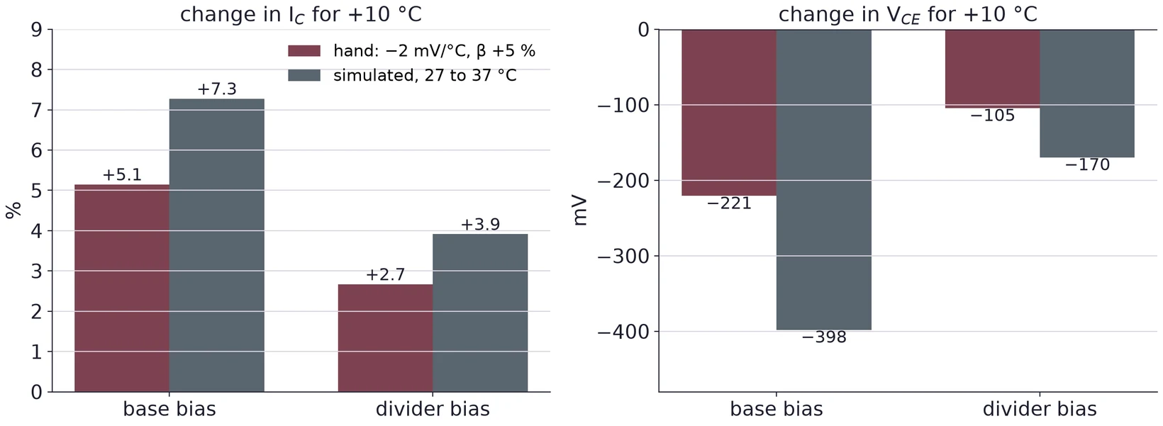
The simulation shows the same order: +7.3 % for base bias and +3.9 % for divider bias. A hotter transistor that draws more current heats itself further; in power circuits this can run away. Divider bias with an emitter resistor is the usual guard against it.
(a) For your design of Practice 7, estimate the change in and for a 15 °C rise, with −2 mV/°C and β up 7 %.
(b) In Task 5, drops by 60 mV while you hold the case. Give the coefficient for a 10 °C rise and for an 8 °C rise. How much does your answer depend on the estimate?
(c) Why does a larger (more volts across ) make the circuit less sensitive to the change in ?
10 Error Analysis for Lab 5
Every task needs an error analysis: for each value, state its uncertainty, name the main sources, and compare it with your design, your simulation or the datasheet.
10.1 A current from a voltage and a resistance
combines two measurements, so their relative errors add in quadrature:
Suppose the manual gives ±(0.5 % + 2 counts) on the 6.000 V range and, as in Lecture 01, ±(0.8 % + 2 counts) on the 6.000 kΩ range. You read = 0.809 V and measure = 1.000 kΩ out of circuit.
= 0.005 × 0.809 + 0.002 = 0.0060 V (0.75 %), and = 0.008 × 1.000 + 0.002 = 0.010 kΩ (1.0 %). So = % = 1.25 %, and = 0.809 ± 0.010 mA.
These numbers are an example; use your own meter's specification for the ranges you used. If you used the color-code value of a ±5 % resistor instead of measuring it, the 5 % dominates everything else.
10.2 β and the base current
is a quotient, so Equation (10) applies again with and . With known to about 1 % and measured directly to 2 %, β is good to about 2.2 %. With from , it is not good to anything (§8.2): say so in your report if that is the method you used, and give the uncertainty you get.
When you compare β with the datasheet, compare with the range at your collector current, and remember that β also depends on temperature and on .
10.3 VCE and the active-region check
is a difference too, but of two values that are not nearly equal, so its error stays small. Measuring directly from collector to emitter avoids the subtraction. The active-region check is a margin, not a precise value: a of several volts is active whatever the meter's last digit says.
10.4 The temperature coefficient
is the difference of two readings on the same range a few seconds apart, so the meter's gain error cancels and only the counts and the drift of the reading remain. The big uncertainty is : without a thermometer, an estimate of 10 °C could easily be off by 3 °C, which is 30 % of the coefficient. State how you estimated , and give the coefficient with that uncertainty. Also note how long you held the case: the reading keeps moving until the transistor stops warming.
10.5 Main sources, task by task
| Measurement | Main error sources |
|---|---|
| Diode-test readings | The meter's test current (readings differ between meters); a hand on the leads; which pair you call C and E |
| Node voltages , , | DMM specification; the supply setting; the meter's input resistance on high-resistance nodes |
| , from drops | Resistor values (measure them); DMM specification on both ranges |
| and β | The subtraction trap; meter burden in series; β's dependence on current and temperature |
| Compared with the design | not 0.7 V; β; E24 rounding; resistor tolerance |
| Temperature coefficient | The estimated ; heating time; drift of the reading |
A difference between measured and expected only means something when it is larger than the uncertainty. When it is, name the source that most likely explains it and check that the size fits.