1 Where Lab 6 Sits
Lab 6 has two halves. First you bias a 2N3904 with a voltage divider, as in Lab 5, and check that it sits in the active region. Then you add three capacitors and a signal, and the biased transistor becomes a common-emitter (CE) amplifier. Last, you connect loads to its output and watch the gain change.
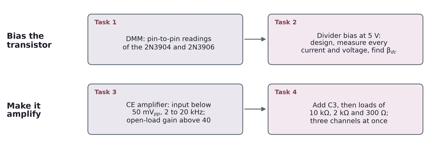
1.1 Task map
| Lab 6 task | What you do | Concept & section |
|---|---|---|
| 1 | DMM readings between every pair of pins of a 2N3904 and a 2N3906 | The junction check (§2.1, and the Lecture 05 notes) |
| 2 | Design a divider bias at 5 V; measure every current and voltage; find | The bias rules (§2) |
| 3 | Build the CE amplifier; measure amplitude, DC offset, phase and the open-load gain | Capacitors (§3), the amplifier (§4), gain (§5), input (§6), measuring (§9) |
| 4 | Add and three loads; show , and together | Loading (§7), swing (§8), measuring (§9) |
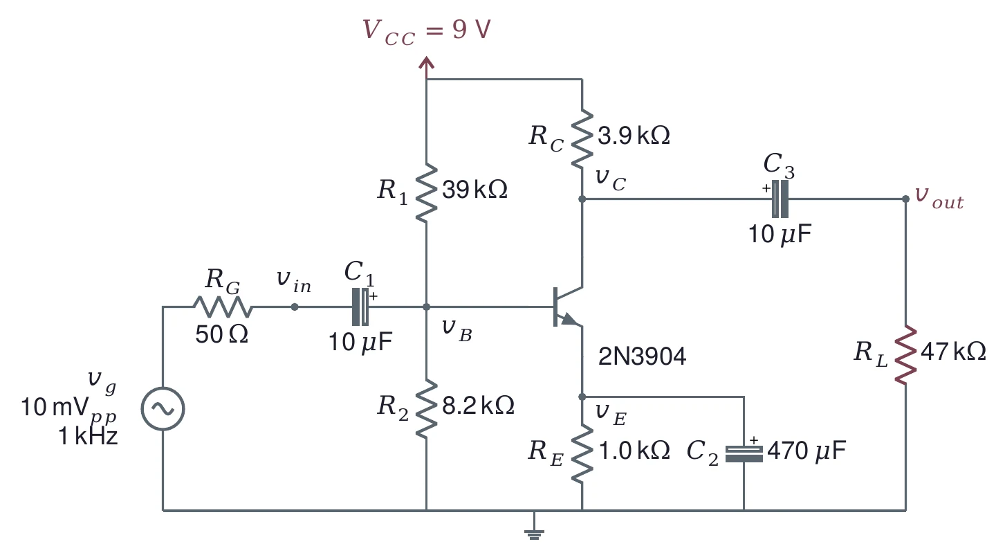
The examples here use one circuit from start to end: = 9 V, = 39 kΩ, = 8.2 kΩ, = 3.9 kΩ, = 1.0 kΩ and a 2N3904. Lecture 05 designs it step by step. Your lab circuit runs from 5 V, so every number in it is yours to work out. Every task needs an error analysis; Section 10 collects the main error sources.
2 The Bias, in Brief
2.1 Task 1: the junction check
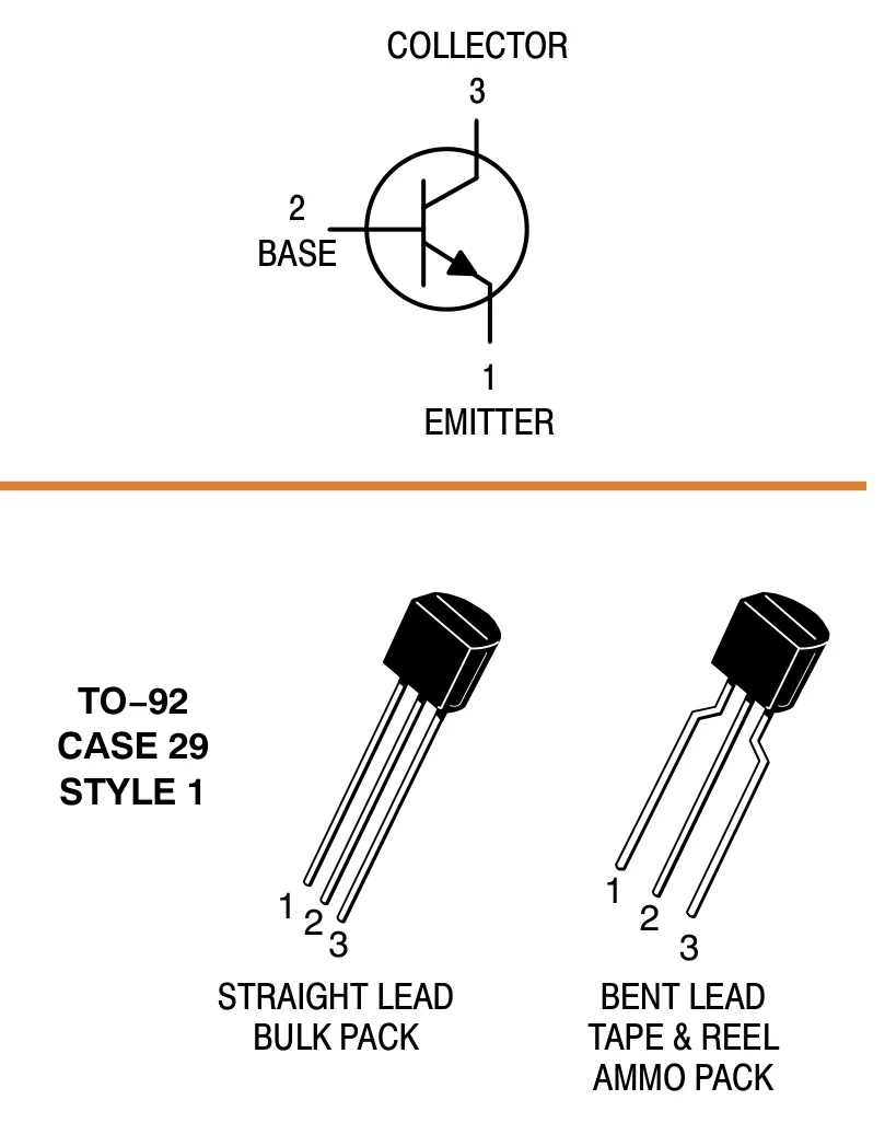
Task 1 is the same DMM table as Lab 5 Task 1. The Lecture 05 notes explain the method and what each pair of leads should show for an NPN and a PNP transistor. You need the pinout to read your table, so here it is again.
2.2 Five rules for divider bias
Task 2 gives you the design rules. Each one has a reason, and knowing the reason tells you how hard to push it.
| Rule | Shared circuit at 9 V (β = 150) | Why |
|---|---|---|
| 0.83 V (aim 0.9 V) | . When is much larger than the changes in from part to part and with temperature, those changes barely move . | |
| 4.97 V | The collector can swing up and down from the middle. | |
| 6.78 kΩ < 7 kΩ with β = 70 | The divider is firm: the base current barely loads it, so β barely moves . | |
| , better | 192 µA = 0.23 | Divider current does no work; it only drains the supply. |
| every Ω | smallest is 1.0 kΩ | Keeps every current, and the power in each part, small. |
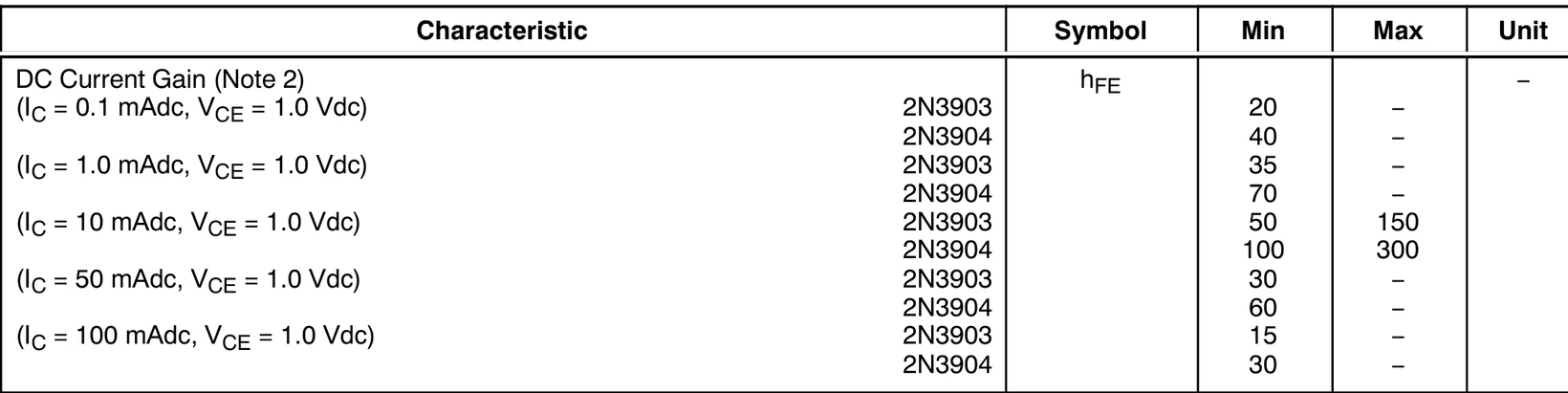
The firm-divider rule uses βdc, and βdc varies a lot from part to part. The onsemi datasheet guarantees only minimums at low current: at 1 mA, and 100 to 300 at 10 mA. Design with the minimum at your current. Then any part from the bag works.
2.3 Two rules pull apart
The firm rule wants a small , which means small resistors. The current rule wants a small , which means large resistors. You can find how much β you need to meet both.
Call , the fraction the divider passes. Then , and
Ignoring , the divider current is . With and , the rule becomes . Put that into the firm rule :
At 9 V, = 0.9 V and = 1.6 V, so = 0.178 and = 0.146. With = 1 (), β must exceed 14.6: easy. With = 0.1 (), β must exceed 146, which is above the datasheet minimum of 70.
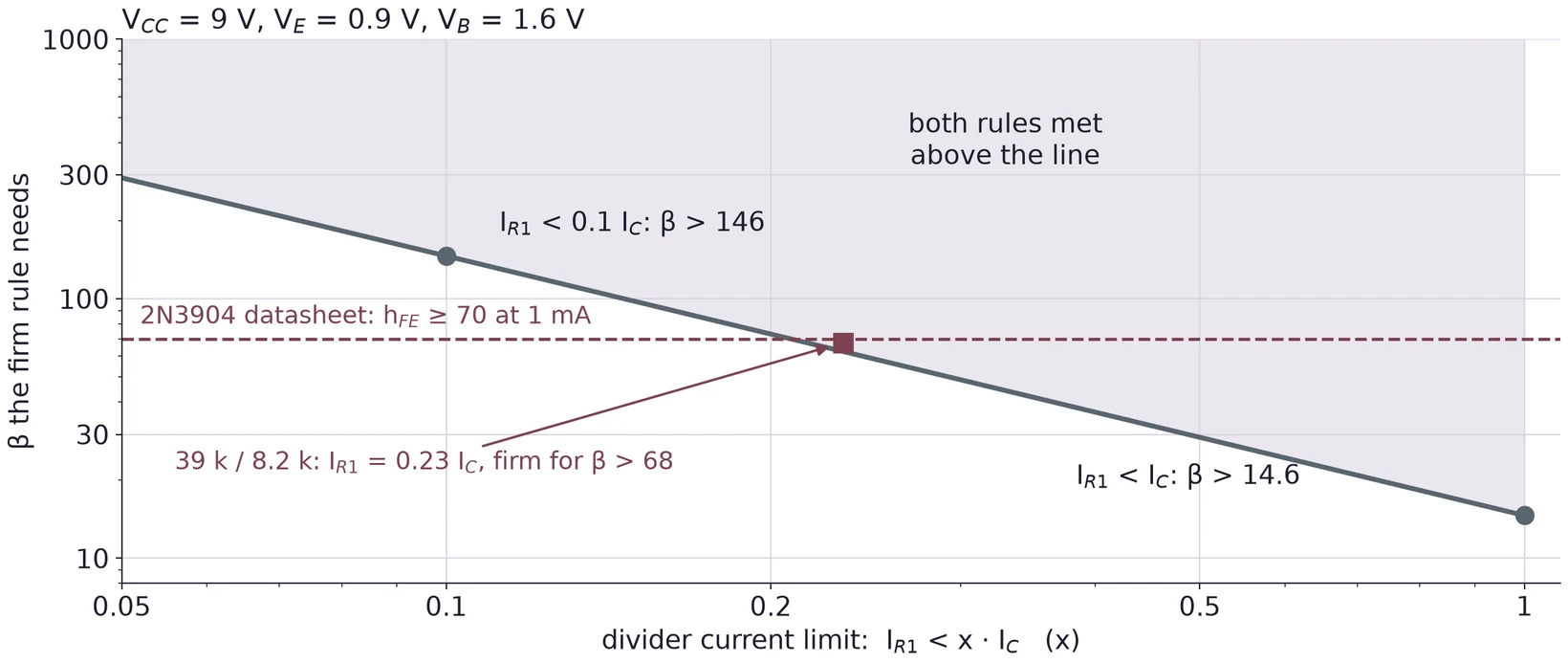
So the "better" half of the current rule often has to give. The shared circuit keeps the firm rule for the worst-case β and accepts a divider current of 0.23 . Work out for your own 5 V design and decide the same way; say in your report which rule you relaxed and why.
2.4 The Q point against β
The base sees the divider as a Thévenin source: behind . The base current flows through , and the emitter current through , so
V and = 6.775 kΩ. With = 0.7 V:
| β | (mA) | (mA) | (µA) | (V) | (V) | (V) |
|---|---|---|---|---|---|---|
| 70 | 0.788 | 0.777 | 11.1 | 0.788 | 5.97 | 5.18 |
| 150 | 0.8265 | 0.821 | 5.47 | 0.826 | 5.80 | 4.97 |
| 300 | 0.8445 | 0.842 | 2.81 | 0.845 | 5.72 | 4.87 |
| ideal divider | 0.864 | 0.864 | 0 | 0.864 | 5.63 | 4.77 |
A fourfold change in β moves by 8 %. The divider current is = 192 µA at β = 150, which is 0.23 : it meets and not , as §2.3 predicted.
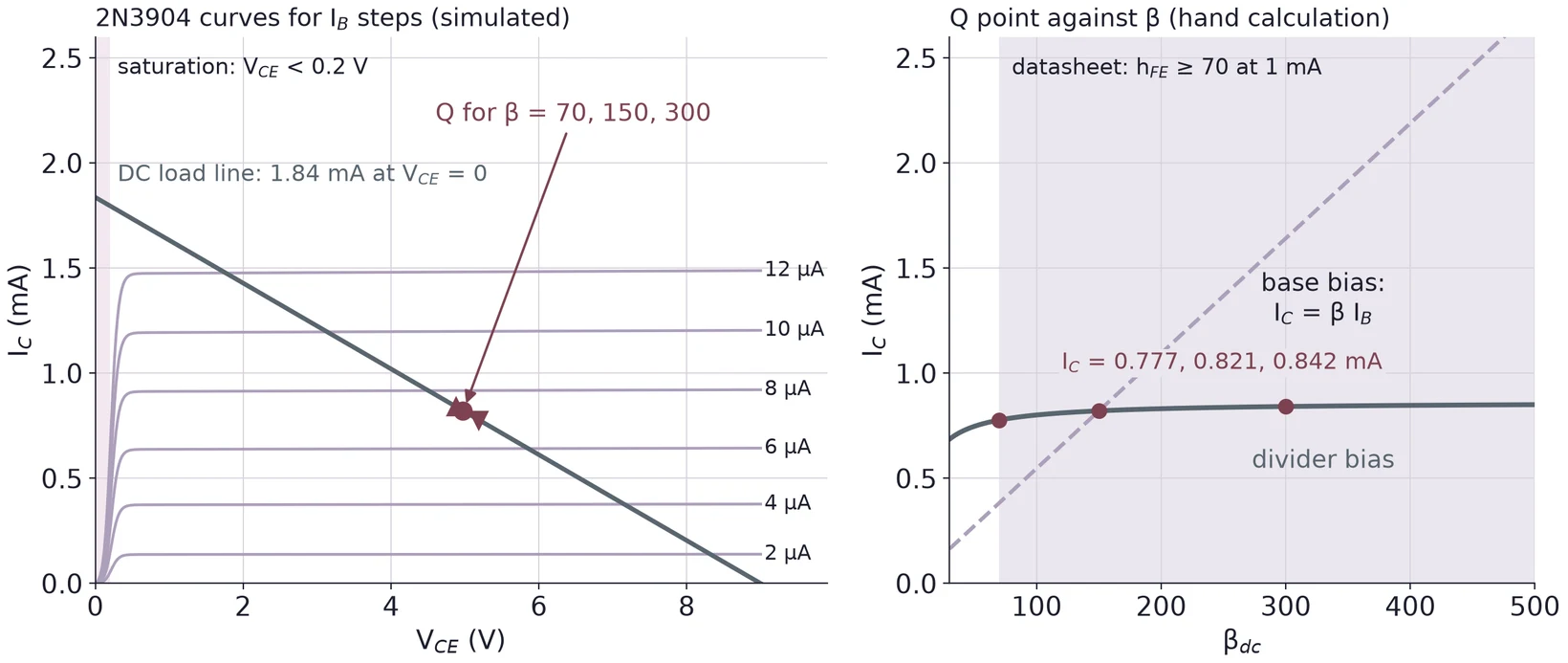
The DC load line joins = 1.84 mA at = 0 and = 9 V at = 0. Every Q point of this circuit lies on it. To check that the transistor is active, not saturated, compare with the datasheet's V (at 10 mA, = 1 mA). At 4.97 V the shared circuit is far from it.
The simulated curves come from onsemi's model, whose βdc is about 114 near 0.9 mA. That is one particular part; yours will differ, and Task 2 asks you to measure it.
(a) Design for = 15 V with = 2.2 kΩ and . Find , the that puts near 7.5 V, and the largest that is firm with β = 70.
(b) For the design in (a), find and the β that the firm rule and need together.
(c) For the shared 9 V circuit, find and with β = 100.
3 Coupling and Bypass Capacitors
3.1 A capacitor passes AC and blocks DC
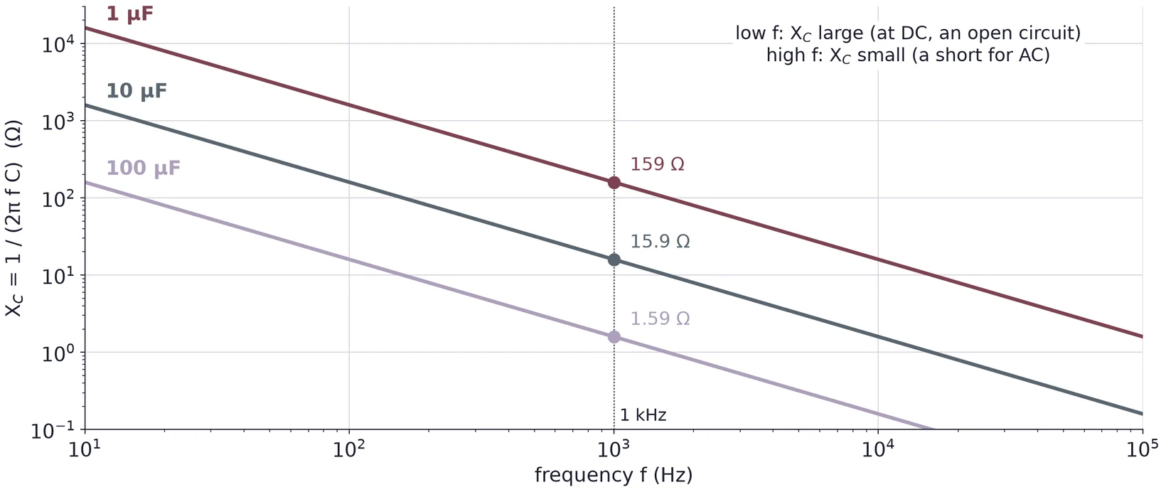
A capacitor's opposition to AC is its reactance,
As rises, falls, and at high enough frequency the capacitor acts as a short. As falls, rises; at DC ( = 0) no current flows through it at all, so it is an open circuit. The amplifier uses both ends of this: the capacitors pass the signal and block the bias voltages.
3.2 The coupling capacitor is a high-pass filter
joins the generator to the base. The base sits at a DC voltage set by the divider, and the generator sits at 0 V DC. Wired straight together, the generator would pull the base away from its bias. In series, blocks the DC and lets the signal through. Seen from the signal, and the resistance after it form a high-pass filter:
where is the whole resistance in the loop: for , the generator's plus the stage's input impedance (§6). At the signal is down to 70.7 %. Well above it passes almost whole.
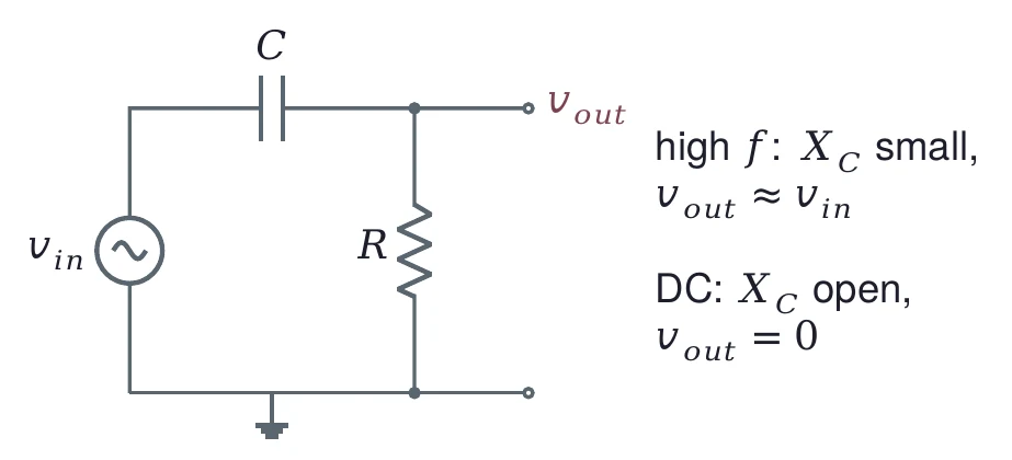
, between the collector and the load, does the same job at the output. The collector sits near 5.8 V DC, and the load should see only the signal.
3.3 The bypass capacitor grounds the emitter for AC
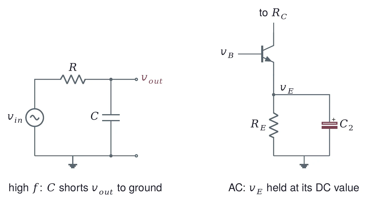
sits across . Seen alone, a resistor feeding a capacitor to ground is a low-pass filter: at high frequency the capacitor shorts the output to ground. At the emitter, that is the point. stays in the circuit for DC and holds the bias steady, while for the signal the emitter is tied to ground. Section 5.4 shows what happens to the gain without it.
3.4 Sizing the capacitors
A simple rule makes each capacitor a short at the lowest frequency you care about: make less than a tenth of the resistance in its loop at that frequency. That puts the corner frequency a decade below the band.
Take 1 kHz as the lowest frequency, a 50 Ω generator and, for the worst case, a 470 Ω load.
. The loop is = 50 + 2717 = 2767 Ω. Ω at 1 kHz needs = 0.58 µF. With 1 µF, = 57.5 Hz; with 10 µF, 5.75 Hz.
. The emitter sees (§5), 30.25 Ω. Ω needs µF. More exactly, the emitter sees = 29.7 Ω, so 100 µF gives a corner at 53.6 Hz and 470 µF at 11.4 Hz.
. The loop is = 3900 + 470 = 4370 Ω. Ω needs µF. With 1 µF, = 36.4 Hz; with 10 µF, 3.64 Hz.
is by far the largest, because the resistance it must beat is the smallest. The simulations in this unit use = 10 µF, = 470 µF and = 10 µF. For your lab, size them for the lowest frequency of the band Task 3 gives.
3.5 Electrolytic capacitors have a + lead
Values of 10 µF and up are usually aluminium electrolytic capacitors. They are polarized: the + lead must sit at the higher DC voltage, and the voltage across the part must stay below its rating. Put one in backwards and it leaks, heats up and can fail. The case carries a stripe of − signs next to the negative lead, and on a new part the + lead is the longer one.
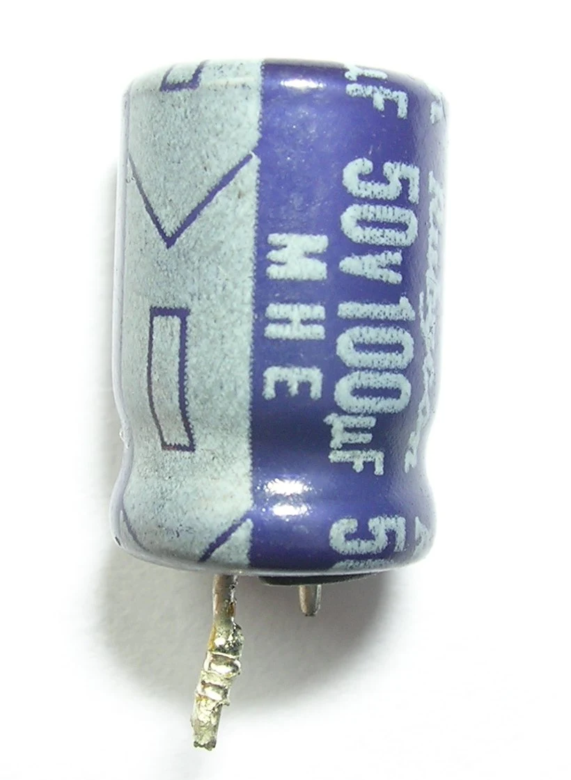

In the shared circuit at β = 150: has 0 V on the generator side and 1.53 V on the base side, so + goes to the base. has 0.83 V on the emitter and 0 V on ground, so + goes to the emitter. has 5.80 V on the collector and 0 V on the load, so + goes to the collector. A 16 V rating covers all three in a 9 V circuit.
(a) A stage has = 1.5 kΩ and is driven from a 50 Ω generator. The lowest frequency is 200 Hz. What is the smallest by the rule? What is with the next larger standard value of 1, 2.2, 4.7 or 10 µF?
(b) The same stage has = 20 Ω. Find the smallest for 200 Hz.
(c) Why does a value of that is too small hurt the gain at low frequency, but not the DC bias?
4 The Common-Emitter Amplifier
4.1 The circuit
Add three capacitors to the biased transistor and it becomes an amplifier. couples the signal into the base, bypasses , and couples the collector to the load. The emitter is tied to AC ground by , so for the signal it is common to the input and the output. That gives the circuit its name.
4.2 DC plus AC at every node
Every node in the amplifier carries a DC voltage from the bias and, on top of it, the signal. Figure 10 shows both at each node, from a simulation with onsemi's 2N3904 model.
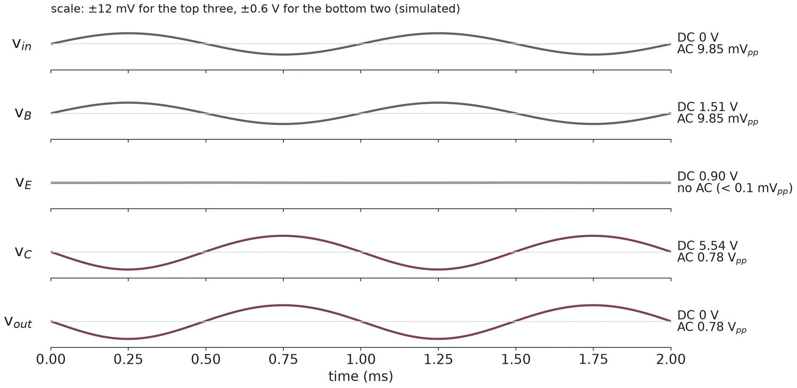
Read it from top to bottom. The signal passes and rides on the base's DC, so is the input on top of 1.51 V. holds the emitter still, so the whole input sits across the base-emitter junction. The junction turns that small voltage into a change of collector current, and turns the current back into a large voltage at the collector. then removes the 5.54 V DC, so the output is centered on zero.
The simulated DC values differ a little from the hand values of §2.4 ( 1.51 against 1.53 V, 5.54 against 5.80 V). The model's is 0.615 V instead of 0.7 V and its βdc is 114, so it runs at 0.888 mA. The same spread shows up between your own calculation and your breadboard.
4.3 The output is inverted
When the base voltage rises, more collector current flows. More current means a larger drop across , so the collector voltage falls. The output is upside down compared with the input: a phase shift of 180°.
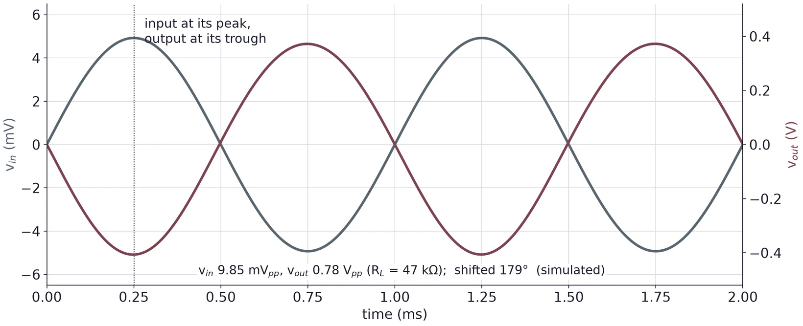
The last degree comes from the coupling and bypass capacitors, whose corners lie between 0.3 and 11 Hz. Each adds a small phase lead well above its corner. At lower frequencies the shift moves further from 180°.
4.4 The AC equivalent circuit
To find the gain, keep only what the signal sees. Two steps turn the amplifier into its AC equivalent:
- Short every large capacitor. Above their corners, is negligible.
- Short the DC supply to ground. A good supply holds its voltage, so it has no AC voltage on it.
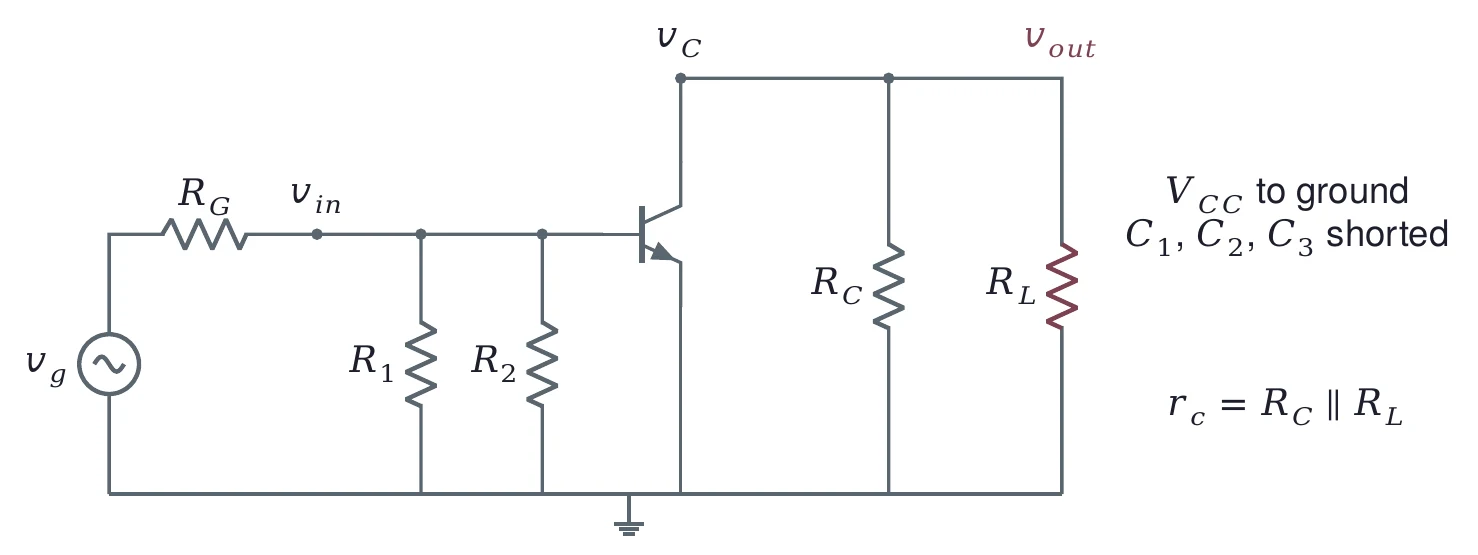
With at AC ground, joins from the base to ground, and joins from the collector to ground. Their parallel value is the AC collector resistance, .
(a) Sketch , and for the shared circuit with removed. Which node gains an AC signal it did not have before?
(b) Draw the AC equivalent of an amplifier whose emitter has two resistors in series, with across only the lower one.
5 r′e and the Voltage Gain
5.1 One current through two resistors
For small signals, the base-emitter junction acts like a small resistor, , in the emitter. The transistor then works as a current source that copies the emitter current into the collector. This picture is the T model.
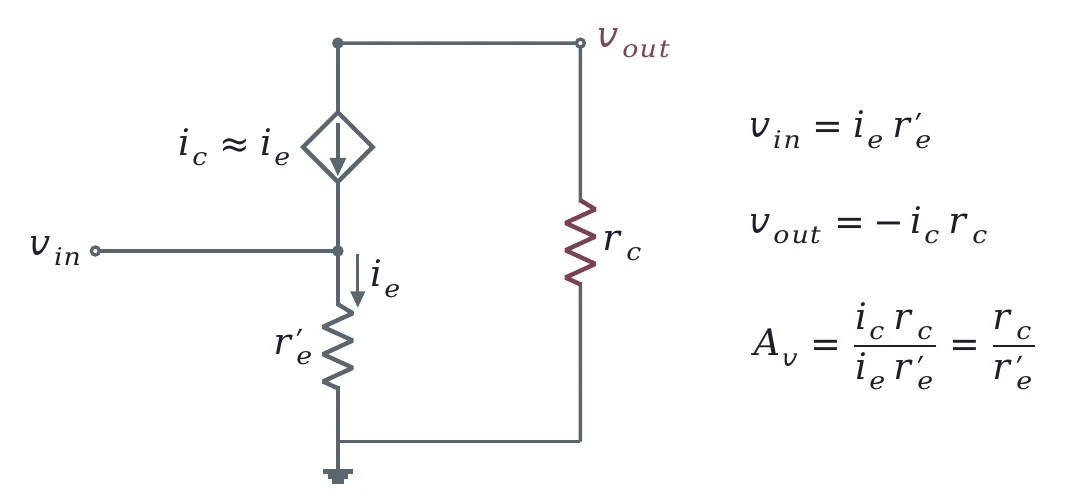
With the emitter at AC ground, the whole input is across : . The same current, less the tiny base current, flows through : . Since ,
The minus sign is the 180° inversion; gains are quoted as magnitudes.
5.2 Where the 25 mV comes from
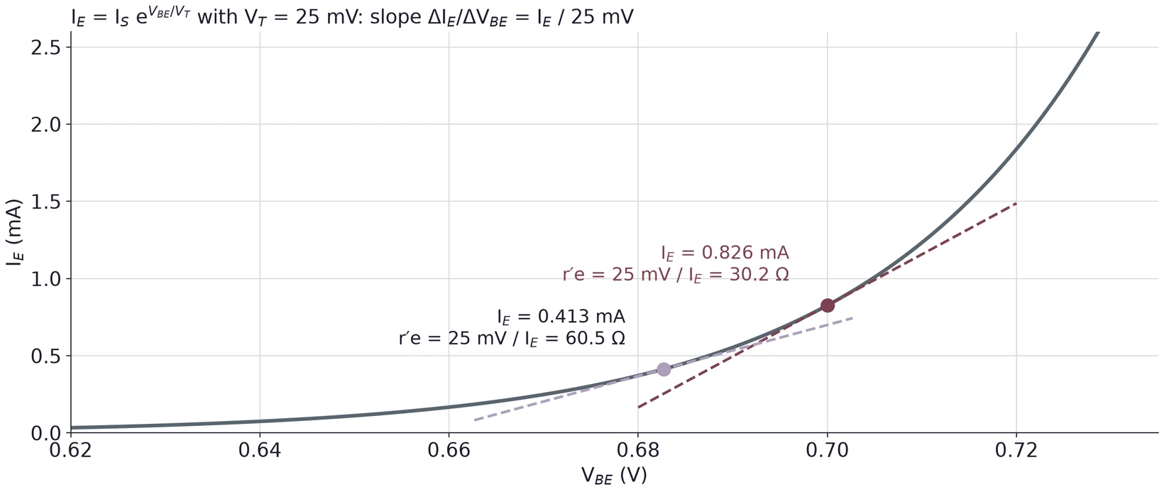
The emitter current of a forward-biased junction rises exponentially with its voltage:
is the thermal voltage: 25.7 mV at 25 °C. A small change of changes along the slope of this curve, and the slope of an exponential is the function divided by its scale:
So is not a part you can buy. It is the slope of the junction curve at the Q point, and it depends only on the current through it: twice the current, half the . Books round to 25 or 26 mV; the difference is 4 %.
5.3 The gain of the shared circuit
With β = 150, = 0.8265 mA (§2.4), so = 25 mV / 0.8265 mA = 30.25 Ω. With no load, = 3.9 kΩ:
With 26 mV instead, = 31.46 Ω and = 124.0. A 10 mVpp input that reaches the base as 9.82 mVpp (§6.3) gives 1.27 Vpp at the collector.
Put into Equation (4) with no load, and use :
The gain of a fully bypassed stage depends only on the DC voltage across . In the shared circuit = 3.20 V, so 128, matching the worked example. With the bias rules of §2.2, is about : 3.6 V at 9 V, a ceiling near 144. Work out the same estimate for your 5 V design before you build it, and compare it with the gain Task 3 asks for.
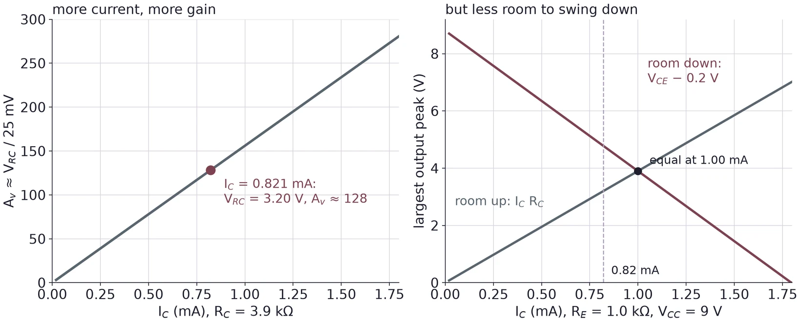
You cannot raise the gain for free. More current means more drop across , so shrinks and the output has less room to swing down before the transistor saturates (§8).
5.4 Without the bypass capacitor
Take out and is back in the emitter for AC. The input now sits across and in series, and
Open load: . With the 47 kΩ load, = 3601 Ω and = 3.50.
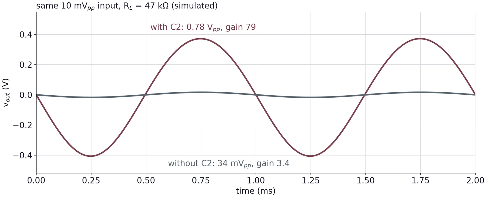
The low gain has a use. It hardly depends on , so it barely changes with temperature or with the signal's size, and the output is less distorted. Many amplifiers leave part of unbypassed for this reason. In Lab 6 the bypassed stage is the one to build.
5.5 The model and the formula disagree
The simulated gain with the 47 kΩ load is 79, while Equation (4) gives 3601/30.25 = 119. The difference is in the model. onsemi's 2N3904 model has an emission coefficient NF = 1.5, which makes its junction curve less steep than the ideal one: its current follows . At its Q point of 0.888 mA, the simulator reports = 22.0 mS, so = 45.4 Ω, against 29.1 Ω for an ideal junction at the same current and 27 °C.
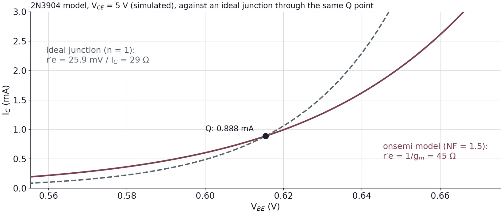
A model is a fit to measurements over a wide range of currents, and this one's slope near 1 mA is not that of an ideal junction. is itself an approximation for an ideal junction. Treat both as estimates: report the formula's gain and the simulated gain next to your measured gain, and say which one your transistor is closer to.
(a) A bypassed stage runs at = 1.5 mA with = 2.2 kΩ. Find and the open-load gain, with 25 mV and with 26 mV.
(b) The same stage with = 680 Ω left unbypassed: what is the gain?
(c) Using Equation (5), estimate the open-load gain of a fully bypassed stage at = 12 V that follows the rules of §2.2.
6 Input Impedance and Source Loading
6.1 Two current gains: DC and small-signal
βdc is the ratio of the DC currents, . For signals, what matters is the ratio of the small changes,
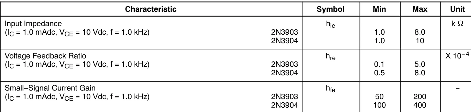
Datasheets call it , with lowercase letters for small-signal values. It is close to βdc but not the same number, because against is not a straight line through the origin. Figure 18 gives the DC gain and Figure 19 the small-signal one. For the 2N3904, onsemi gives at 1 mA and = 100 to 400 at 1 mA, 10 V and 1 kHz.
6.2 The π model: the base sees βr′e
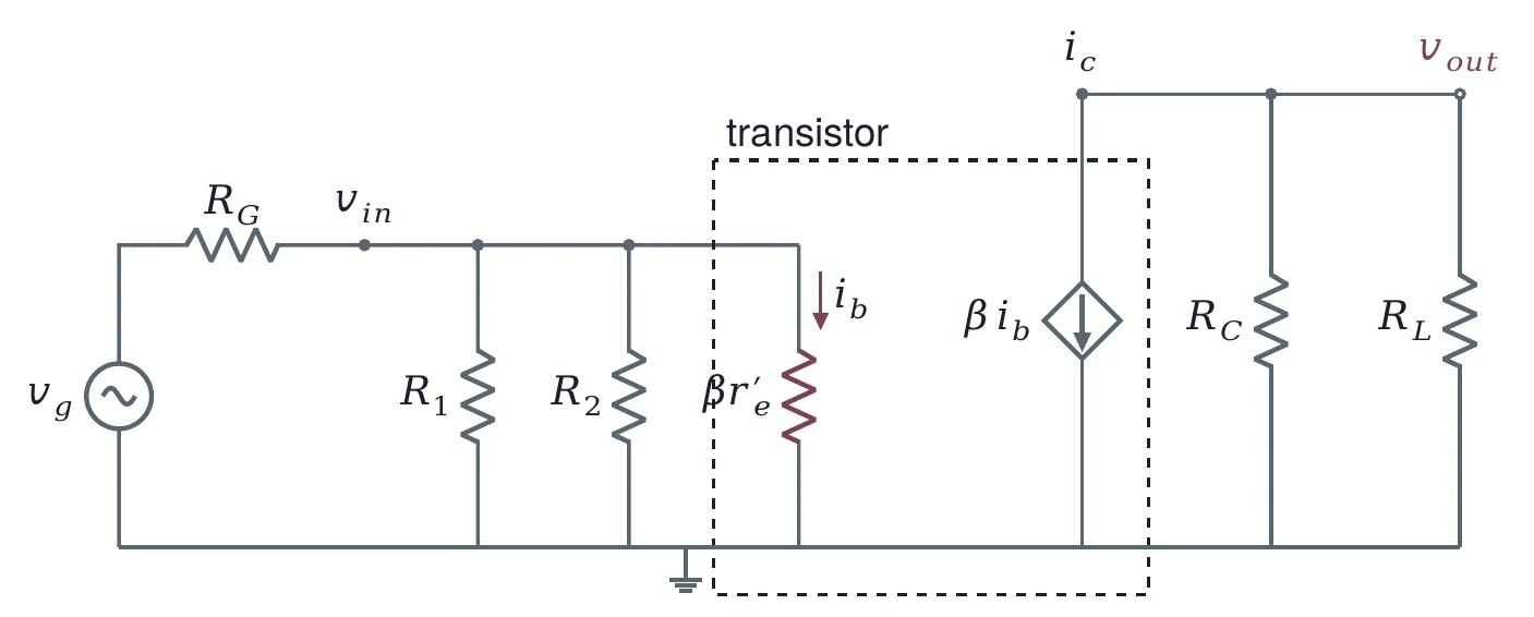
The T model puts in the emitter. Seen from the base, that resistor looks larger. The input voltage drives through , but the base supplies only of it:
The π model draws exactly this: a resistor from the base to ground, and a current source from the collector to ground. It gives the same gain as the T model and makes the input side easy to read.
6.3 The input impedance of the stage
The generator sees three resistances from the base to ground in parallel:
With βac = 150, = 150 × 30.25 Ω = 4537 Ω, and = 6775 Ω. So
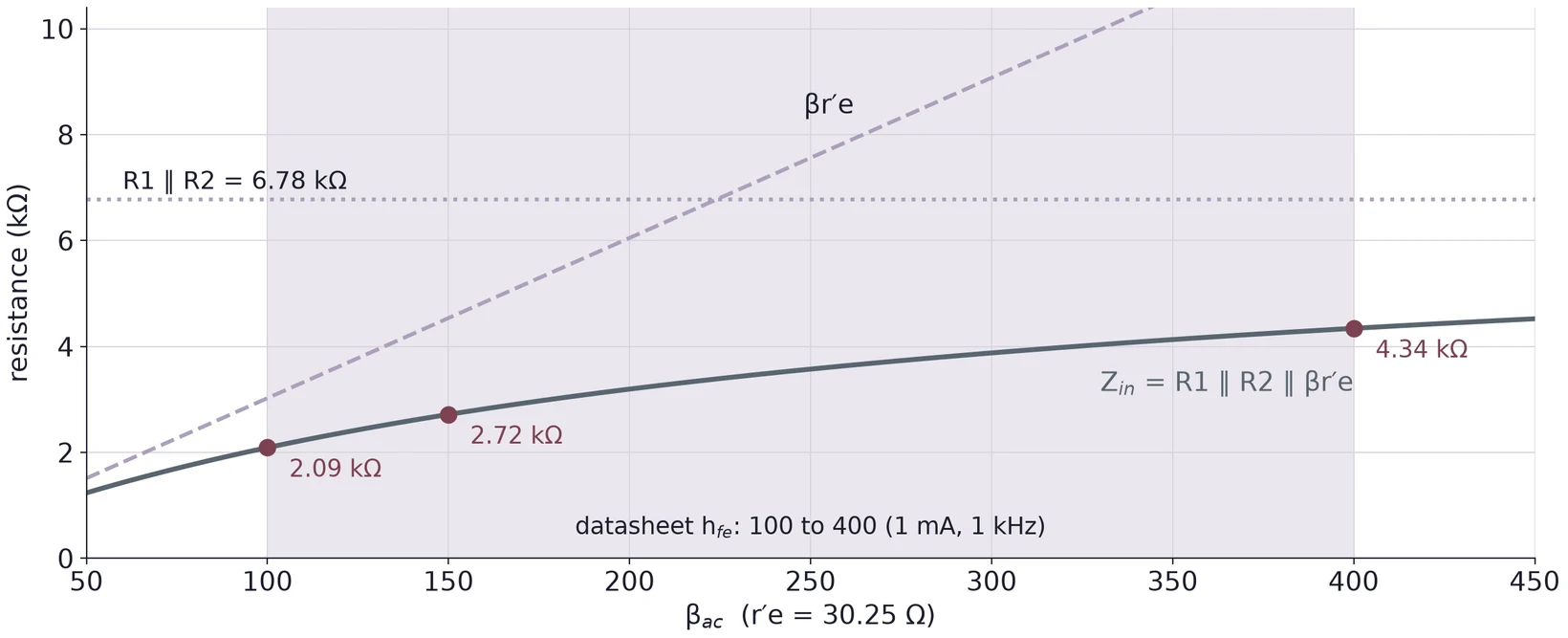
Because βac is uncertain by a factor of four, so is , and follows. Measure it if you need it: put a known resistor in series with the input and see how much of the signal reaches the base.
6.4 The source divides with the input impedance
A function generator is an ideal source behind its output resistance (50 Ω on most lab generators). and form a voltage divider:
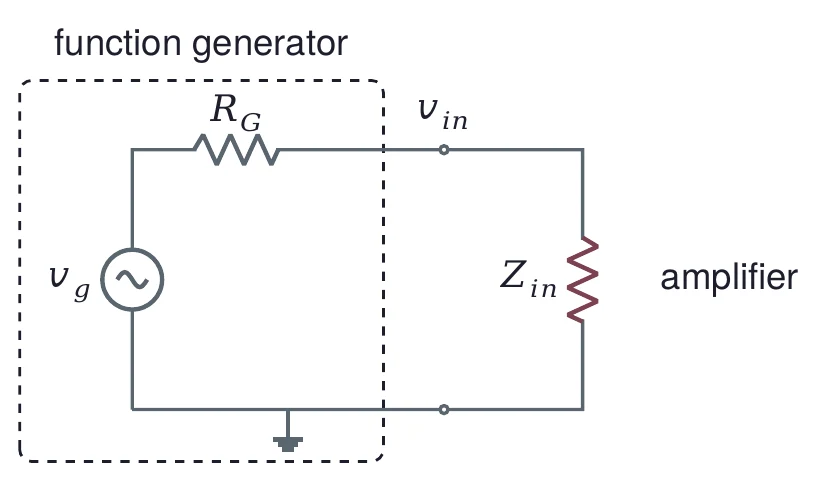
With = 50 Ω: = 2717/2767 × 10 mVpp = 9.82 mVpp, 98.2 %. With a 600 Ω source: 2717/3317 = 81.9 %, 8.19 mVpp. With the 50 Ω generator, the open-load output is 128.9 × 9.82 mV = 1.27 Vpp.
The gain is defined from at the amplifier, not from the number on the generator's display. Measure with the scope, at the input of the amplifier, every time you measure .
(a) For the shared circuit, find and with βac = 250.
(b) A 1 kΩ source drives the shared circuit at βac = 150 with = 5 mVpp. What reaches the base, and what is the open-load output?
(c) Why does raising and by the same factor raise , and what does it cost the bias?
7 Loading the Output
7.1 A load sits in parallel with the collector resistor
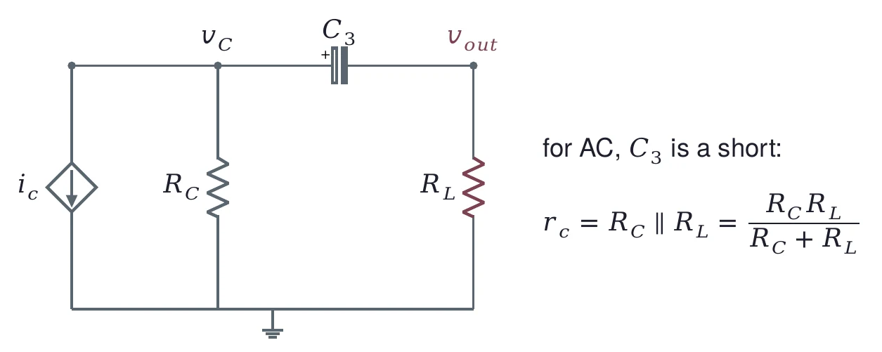
connects the load to the collector. For DC it is open, so the load does not change the bias. For AC it is a short, so the load sits in parallel with , and the AC collector resistance drops to
7.2 Gain falls with the load
With = 30.25 Ω and 9.82 mVpp at the base:
| 47 kΩ | 3601 Ω | 119.1 | 1.17 Vpp |
| 4.7 kΩ | 2131 Ω | 70.5 | 692 mVpp |
| 470 Ω | 419 Ω | 13.9 | 136 mVpp |
| 100 Ω | 98 Ω | 3.2 | 31.7 mVpp |
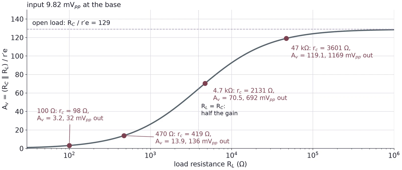
A CE stage has an output resistance of about : seen from the load, it is a source behind 3.9 kΩ, like the loaded divider of Lecture 01. A load much larger than takes nearly the full output. A load much smaller than shorts most of it. That is why a CE stage is often followed by a stage with a low output resistance when it has to drive a small load.
also forms a high-pass filter with . A smaller load lowers that resistance and raises the corner, so check against your smallest load (§3.4).
(a) Find , and for the shared circuit with loads of 22 kΩ and 1 kΩ, for 9.82 mVpp at the base.
(b) With = 1 µF, find the corner frequency for each load in (a).
(c) Which load in (a) gives the most output power, ?
8 Swing, Clipping and Distortion
8.1 How far the collector can swing
The collector sits at its Q point and swings both ways. It cannot go up past the point where reaches zero (cutoff), and it cannot go down past the point where the transistor saturates. For a bypassed stage the emitter stays at , so the collector can fall to about .
Open load, β = 150: the collector can rise by = 0.821 mA × 3.9 kΩ = 3.20 V before = 0. It can fall by V = 4.97 − 0.2 = 4.77 V before saturation. The smaller one, 3.20 V, limits a clean output to 6.4 Vpp. With a load, the upward limit becomes .
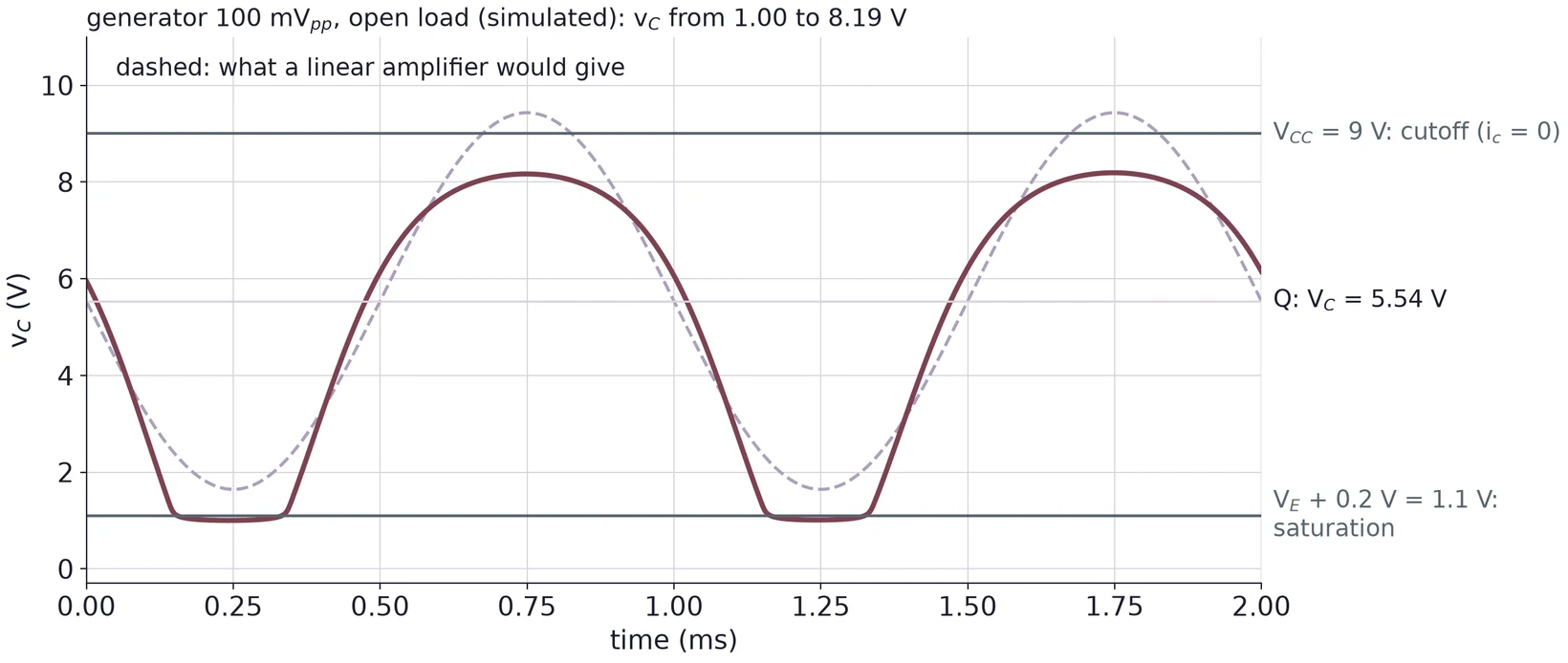
In Figure 25 the bottom is flat: the transistor saturates for part of each cycle. The top is rounded but never reaches 9 V. Before the transistor cuts off, the exponential junction has already squeezed that half of the wave (§8.2).
8.2 Distortion: the junction is not a straight line
is the slope at one point of an exponential curve. A large signal walks along the curve, where the slope changes. With the AC voltage across the junction,
so equal positive and negative swings of give unequal swings of current.
With = 25.7 mV, a sine of 2 mVpp at the base (±1 mV) makes swing from −3.8 % to +4.0 %. At 10 mVpp: −17.7 % to +21.5 %. At 50 mVpp: −62 % to +164 %, far from a sine.
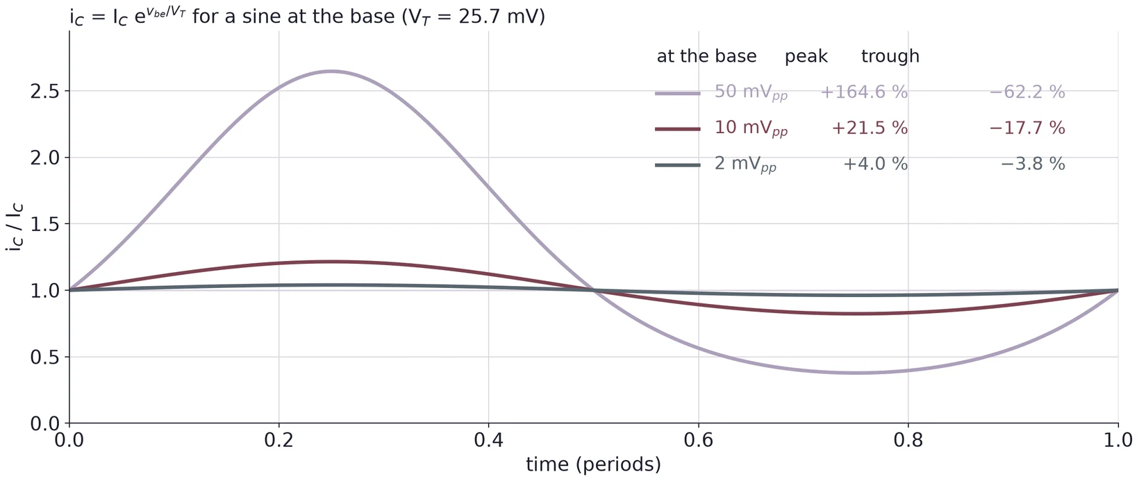
Because the circuit inverts, the tall current peaks pull the collector down, toward saturation, and the shallow troughs let it rise less. Even the 10 mVpp of the worked examples shows a visible difference between the two halves.
8.3 The small-signal rule
A common rule keeps the AC emitter current below a tenth of the DC current: . The voltage across the junction is , so
For a fully bypassed stage this holds whatever the bias, because is always 25 mV. On the bench, start with a few millivolts at the base. Raise the input only while the top and bottom halves of stay the same height. If they differ, the input is too large, and the gain you measure is not the small-signal gain.
(a) A bypassed stage has = 1.2 mA, = 3.3 kΩ and = 4.0 V. Find the room up and down for the open-load output. Which limit sets the largest clean output?
(b) The same stage drives a 10 kΩ load. What is the room up now?
(c) Find the positive and negative swing of , in percent, for 5 mVpp at the base.
9 Measuring with the Oscilloscope
9.1 Offset, amplitude and phase
Task 3 asks for three things about the output: its amplitude, its DC offset and its phase relative to the input. The scope's input coupling decides which you can see.
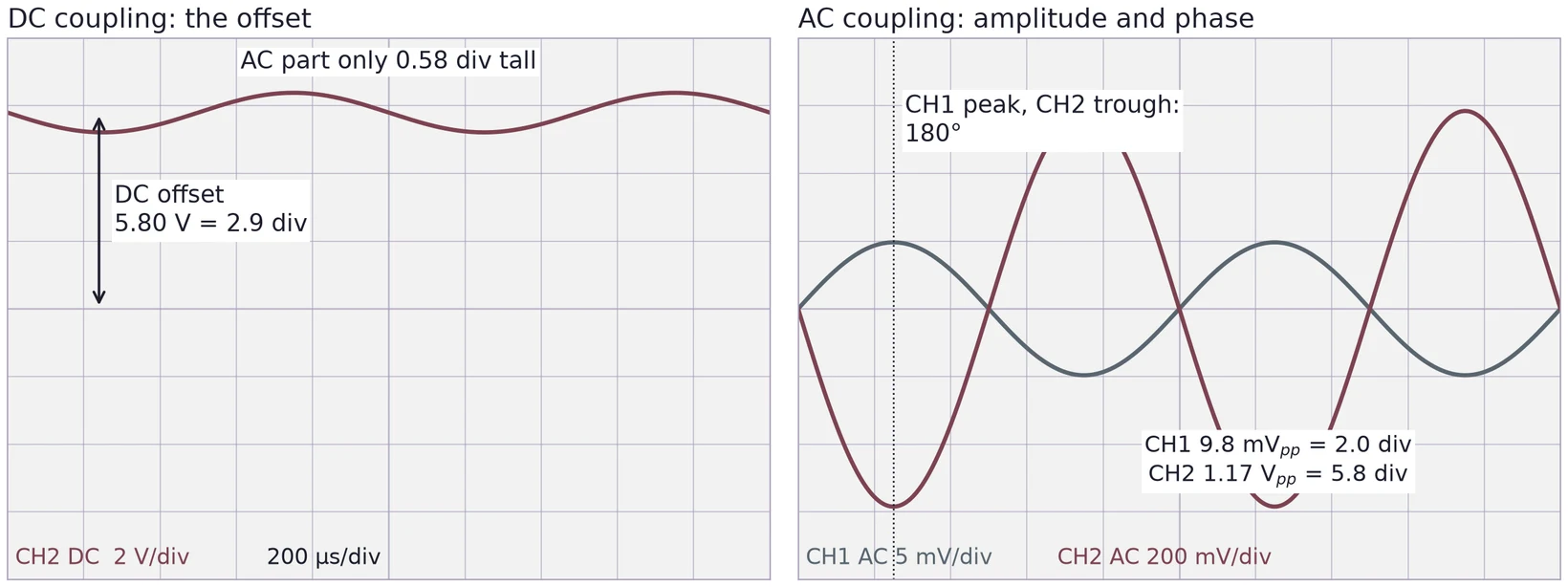
DC offset. With DC coupling, the trace shows the whole voltage, DC plus AC. Read the offset as the height of the trace's center above the ground marker. At it is the collector's Q-point voltage; at , after , it should be close to zero.
Amplitude. With AC coupling, the scope blocks the DC with a capacitor of its own, so you can use a sensitive scale and fill the screen with the swing. Read as in Lecture 01. AC coupling adds a high-pass filter of its own; check in your scope's manual that its corner is far below your signal frequency.
Phase. Put and the output on two channels with the same time base. Measure the time between matching points, such as a positive peak of one and the nearest negative peak of the other, and convert it: phase = 360° × . An inverting stage gives close to 180°.
9.2 Three waveforms at once
Task 4 asks for , and on the screen together. Each probe has a ground clip, and all of them must go to the circuit's ground: on most bench scopes the clips are tied together through the instrument, so a clip on any other node shorts that node.
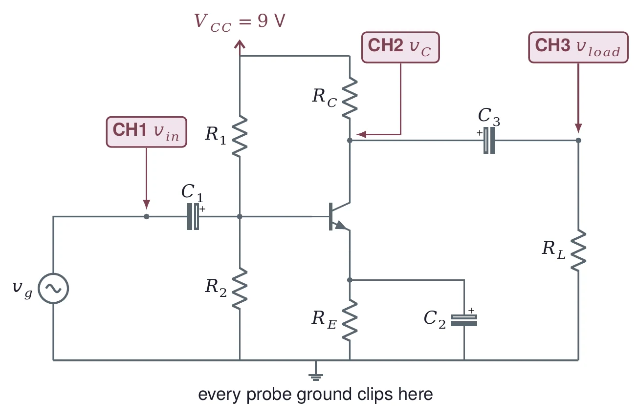
Trigger on CH1, the input, so the picture is stable whatever the load does. Give each channel its own volts per division. Above the corner of , is the AC part of without its DC. A smaller load makes both smaller, because it lowers .
9.3 Small signals are noisy
A few millivolts at the input is close to the noise of a scope channel on its most sensitive range. Use the scope's averaging or its bandwidth limit if it has them, read the amplitude with the built-in measurement rather than by eye, and say in your report which you used. Another way is to measure the generator's larger, cleaner signal and compute from a known divider, but then the divider's tolerance joins your error budget.
(a) On a screen at 10 mV/div, spans 1.6 divisions; at 0.5 V/div, spans 3.4 divisions. Find the gain.
(b) At 200 µs/div and 1 kHz, the input's peak and the output's nearest trough are 0.1 division apart from where 180° would put them. How many degrees is that?
10 Error Analysis
Every task needs an error analysis. For each value you report, state its uncertainty, name the main sources of error, and compare it with the value you expected, simulated or took from the datasheet. Two cases in this lab need care.
10.1 β from the base current
Task 2 asks for and βdc. It is tempting to compute from two currents you already measured. That subtracts two nearly equal numbers, and their errors add.
Suppose your meter reads each current to ±0.5 % and you find = 0.8265 mA and = 0.8210 mA. Then = 5.50 µA, with an uncertainty of
That is 106 % of the value (8.24 µA in the worst case). The difference tells you nothing about β.
Measure directly instead, on the µA range in series with the base. If that reading is 5.47 ± 0.2 µA, then
so βdc = 150.1 ± 5.5.
Use your own meter's specification for the ranges you used. You can also find and without breaking the circuit: measure the voltage across or and divide by the resistor's measured value. Then the resistor's measured value joins the error.
10.2 The gain
Suppose you read = 9.8 ± 0.4 mVpp (noise and trace width at a sensitive scale) and = 1.27 Vpp ± 3 % (the scope's vertical accuracy). Then = 129.6, and
so = 129.6 ± 6.6. The small input is the larger error.
10.3 What to compare with
| Measurement | Main error sources | Compare with |
|---|---|---|
| Bias voltages and currents | Meter specification; resistor tolerance; and β of your part | Your design calculation; a simulation |
| βdc | The reading above all | Datasheet at your current |
| Open-load gain | Reading ; scope accuracy; input too large (distortion) | ; mV; a simulation |
| Loaded gain | The same, plus the load's tolerance | |
| Phase | Reading ; capacitor corners near your frequency | 180° |
Temperature also moves the gain. is 25.26, 25.69, 26.12 and 26.55 mV at 20, 25, 30 and 35 °C, so , and with it the bypassed gain, changes by about 1.7 % for every 5 °C. A transistor warmed by your fingers, or a bench lamp, can shift a reading by that much. A difference between measured and expected only means something when it is larger than the uncertainty. When it is, say which source most likely explains it, and check that the size fits.
(a) You read = 4.0 ± 0.2 mVpp and = 0.50 Vpp ± 3 %. Find and its uncertainty.
(b) Your measured open-load gain is 20 % below . Name two causes from this unit that could explain it, and a measurement that would tell them apart.