Part 1 · Lab 6 in four tasks
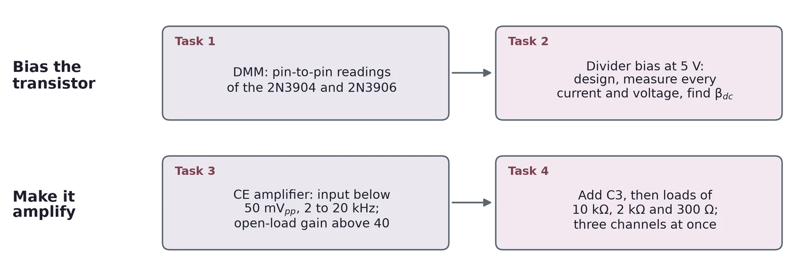
Tasks 1 and 2 bias a 2N3904, as in Lab 5. Tasks 3 and 4 turn the biased transistor into an amplifier and load it.
Task 1 repeats Lab 5's junction check
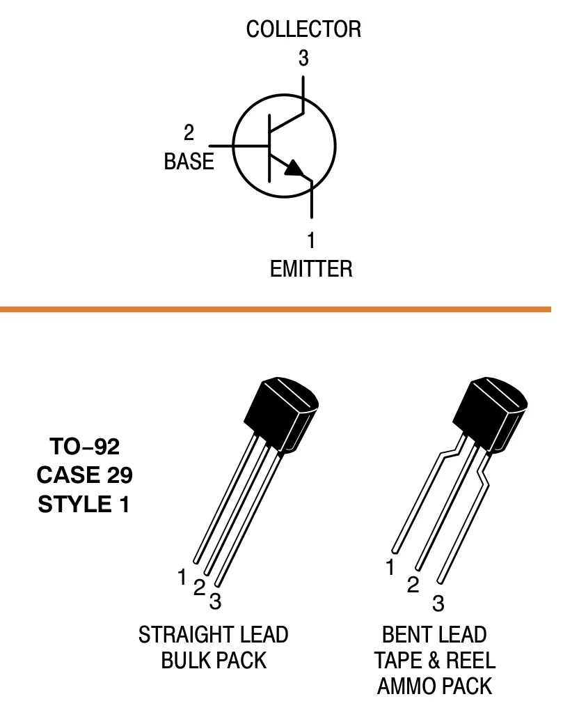
The same DMM table as Lab 5 Task 1: six lead pairs, for the 2N3904 and the 2N3906.
The method and what each pair should show are in the Lecture 05 notes.
Pins 1, 2, 3 are emitter, base, collector.
onsemi 2N3903/D datasheet (Rev. 9), p. 1: TO-92 pinout.
Two divider rules pull apart
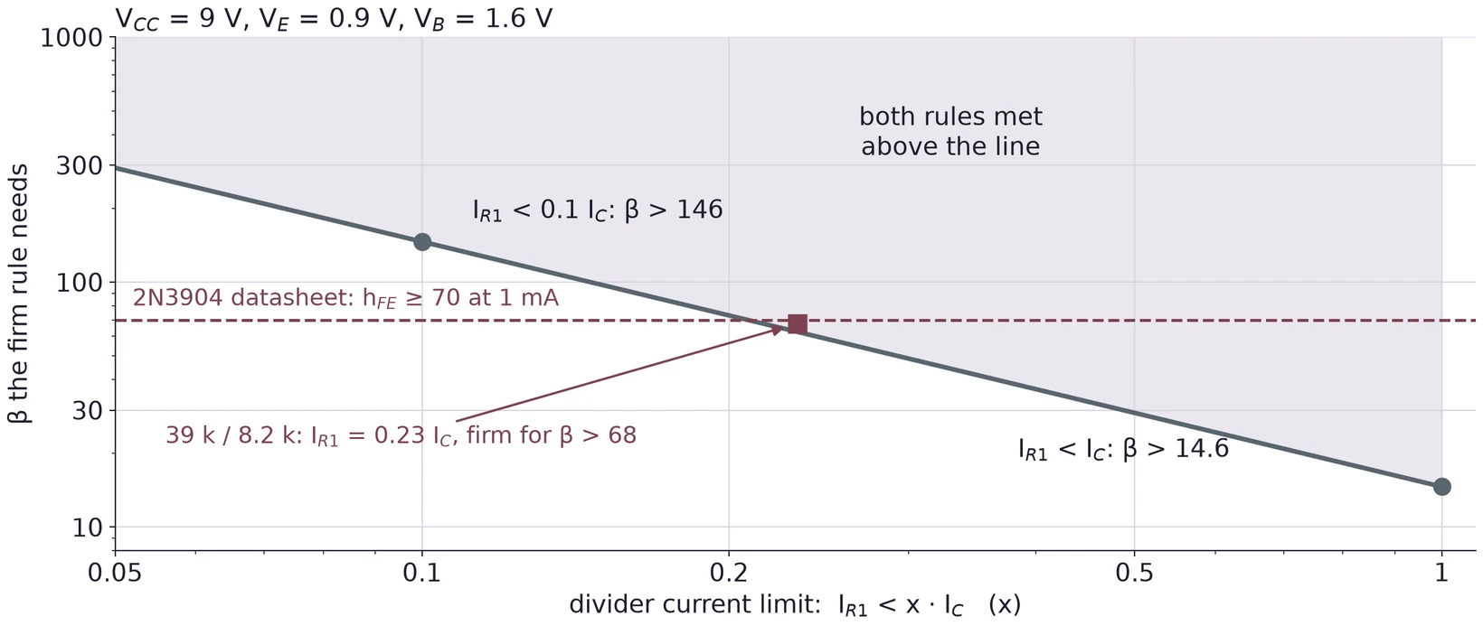
A firm divider wants small resistors; a small divider current wants large ones. At 9 V, and a firm divider together need β above 146.
Divider bias holds the Q point when β changes
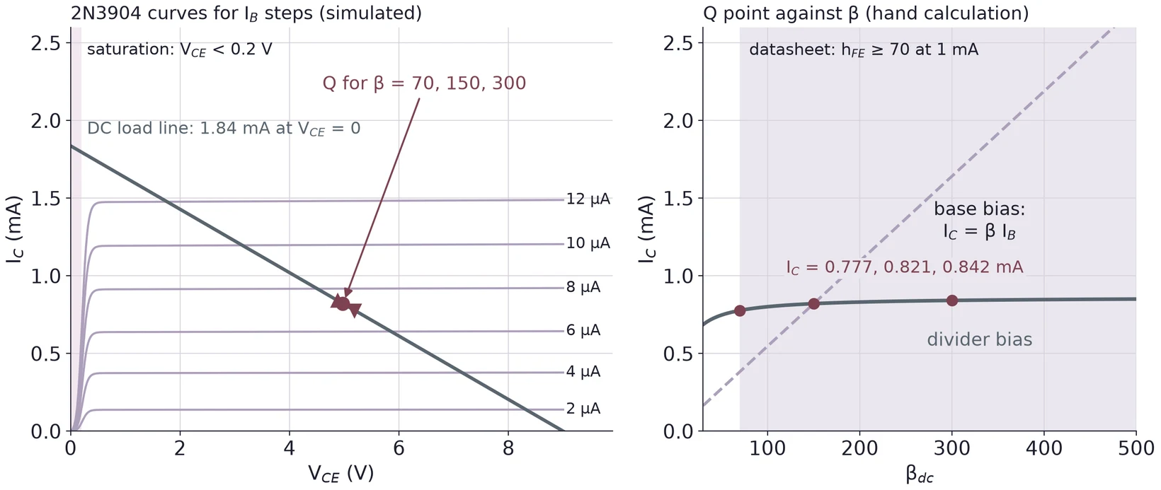
β from 70 to 300 moves from 0.777 to 0.842 mA and from 5.18 to 4.87 V: active, far from saturation. Base bias would follow β.
Part 2 · A capacitor passes AC and blocks DC
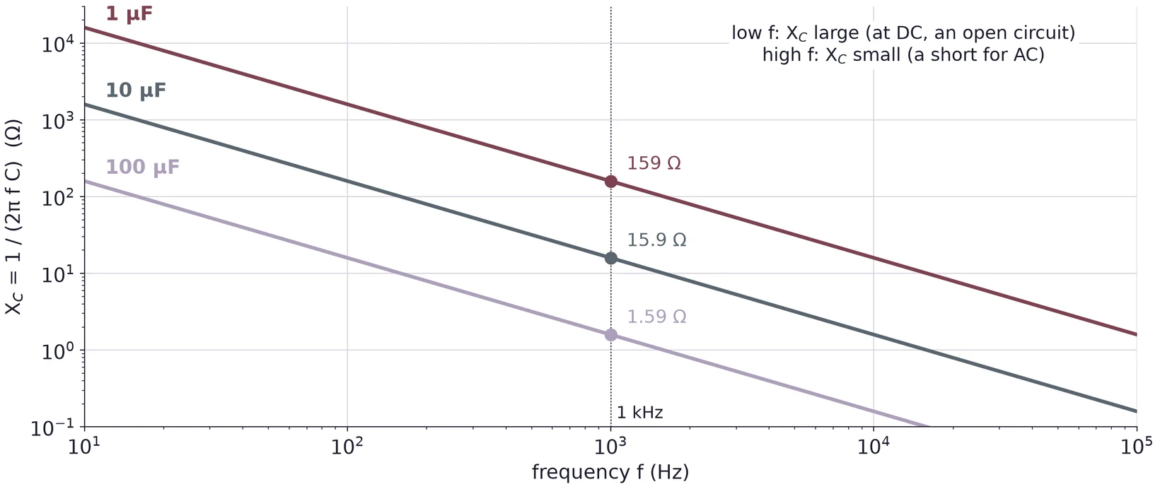
. As rises, falls toward a short. As falls, rises toward an open.
The coupling capacitor is a high-pass filter
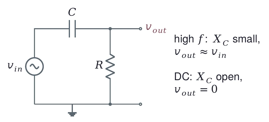
= 1 µF into = 2.77 kΩ:
= 57.5 Hz
With 10 µF: 5.75 Hz
The signal passes; the base's DC (1.53 V) does not leak back into the generator. = 2.72 kΩ comes in Part 4.
The bypass capacitor grounds the emitter for AC
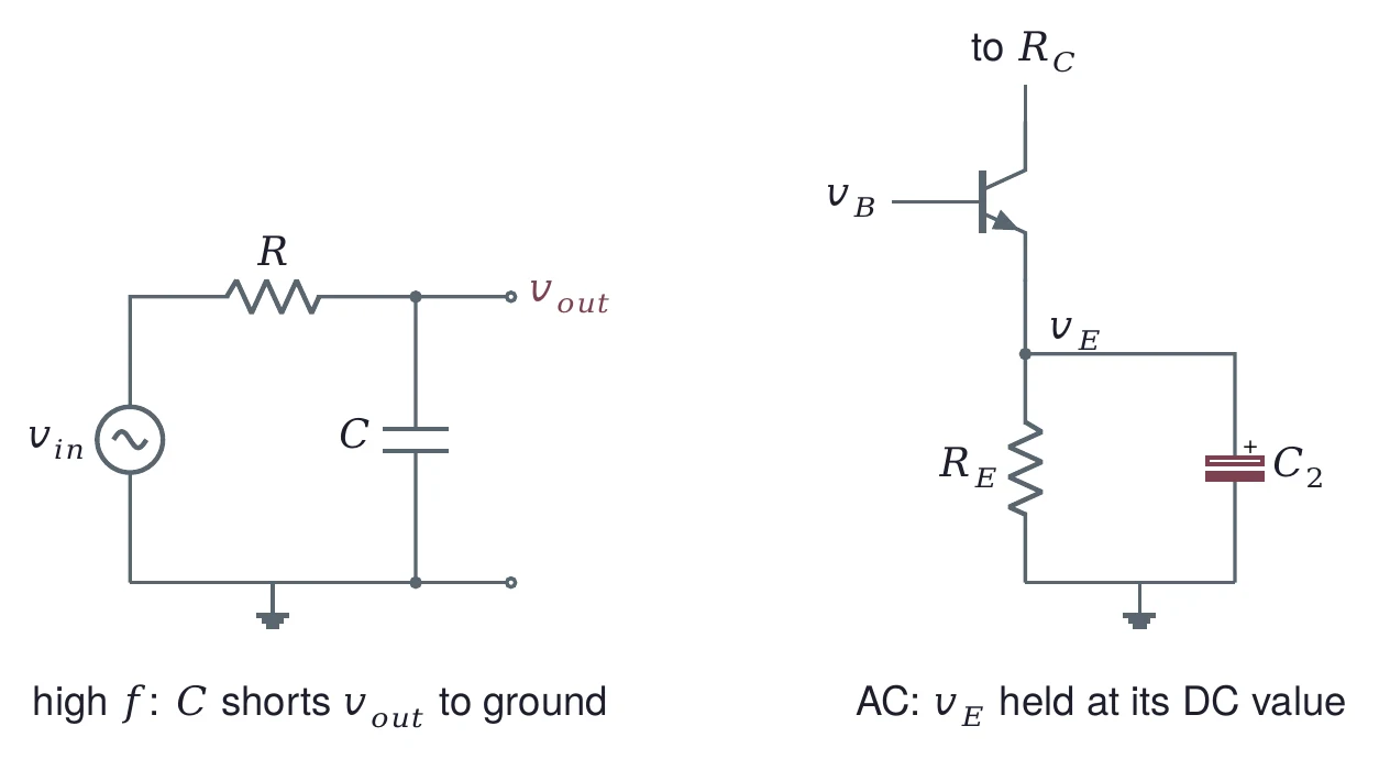
The same capacitor seen as a low-pass filter: above its corner, holds the emitter at its DC voltage, so for AC the emitter is ground.
Electrolytics: + goes to the higher DC side
| C | DC on each side | + lead to |
|---|---|---|
| generator 0 V, base 1.53 V | base | |
| emitter 0.83 V, ground 0 V | emitter | |
| collector 5.80 V, load 0 V | collector |
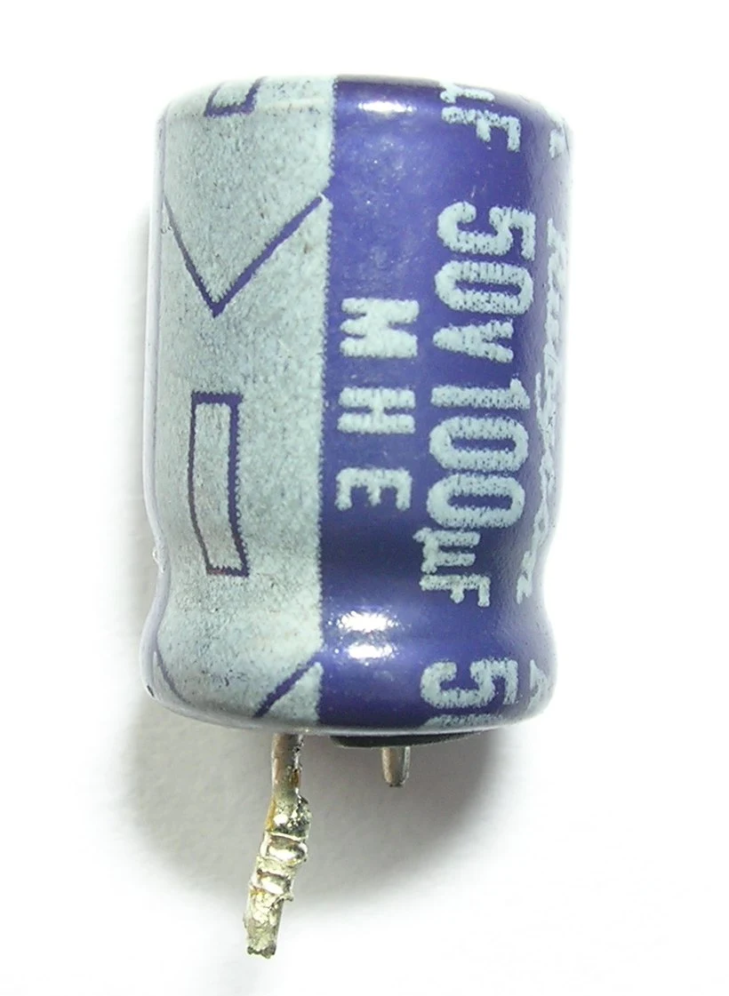
The stripe of − signs marks the negative lead.
Pick a voltage rating above the DC across it. Photo: Willtron, CC BY-SA 3.0.

Part 3 · The common-emitter amplifier
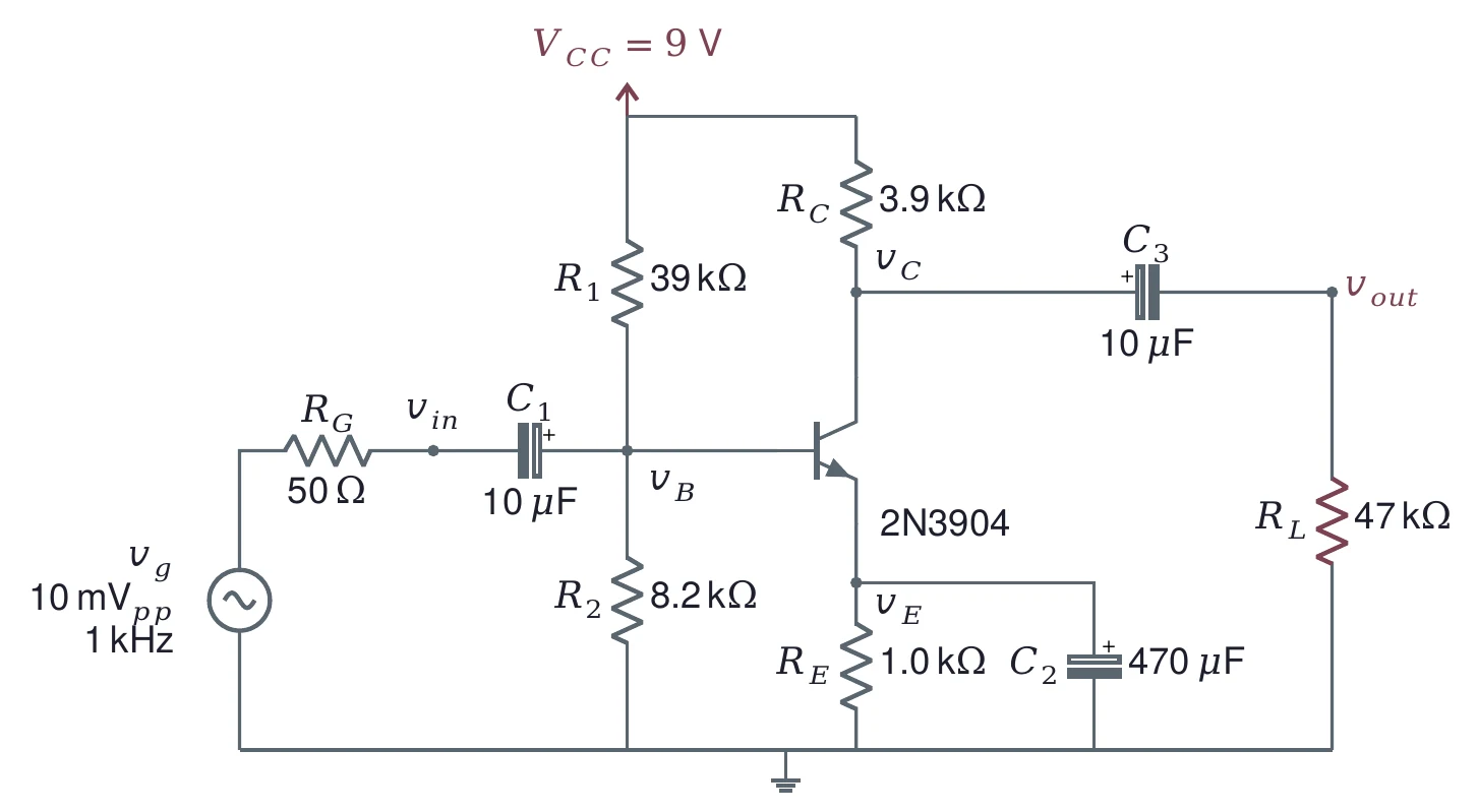
The bias network of Part 1 plus three capacitors. The emitter is AC ground, common to input and output.
DC plus AC at every node
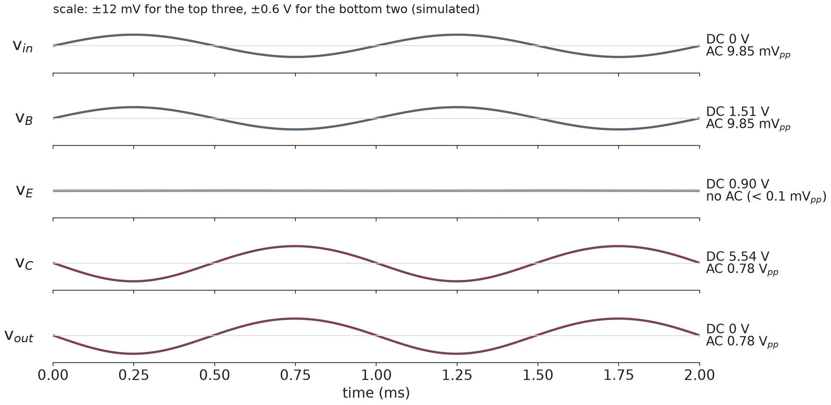
Simulated (onsemi 2N3904 model, 10 mVpp at 1 kHz). has no AC: holds it. strips the 5.54 V DC from the output.
The output is inverted
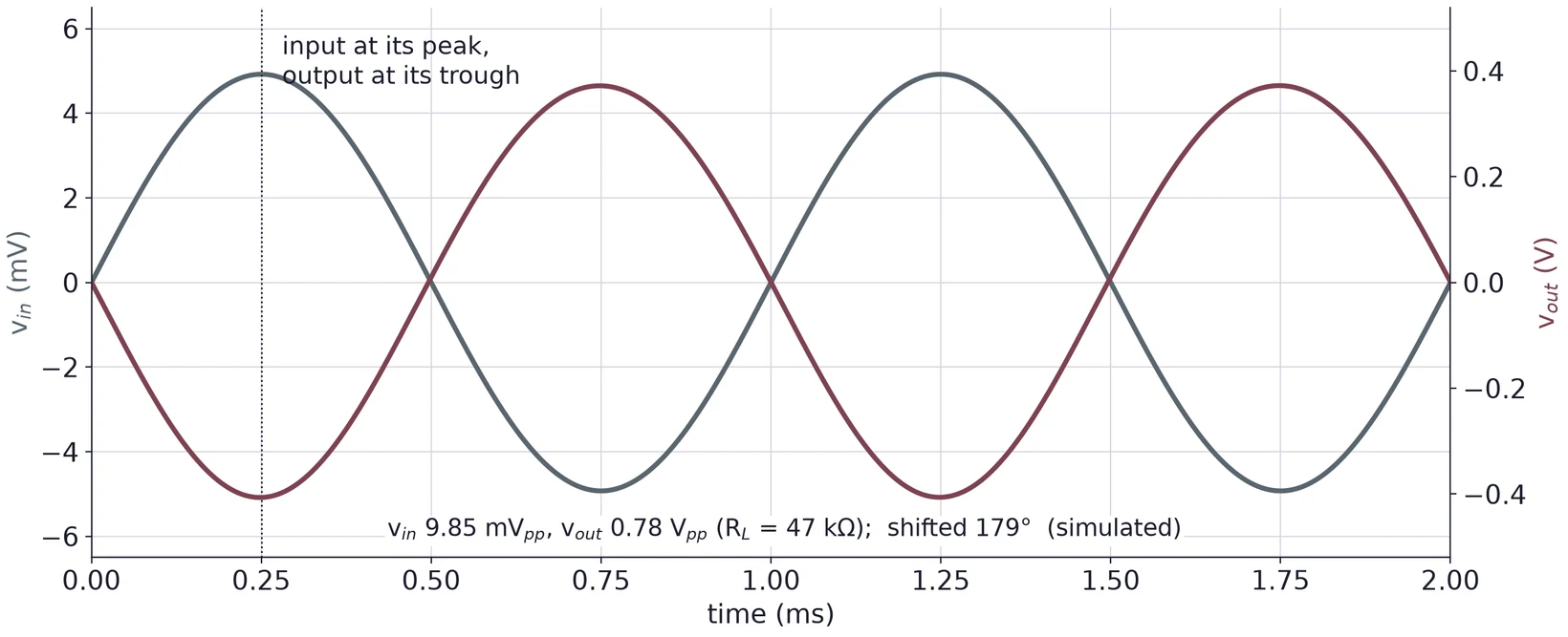
Base up, more , more drop across , so goes down. Simulated: 179° at 1 kHz; the coupling capacitors add the last degree.
The AC equivalent circuit
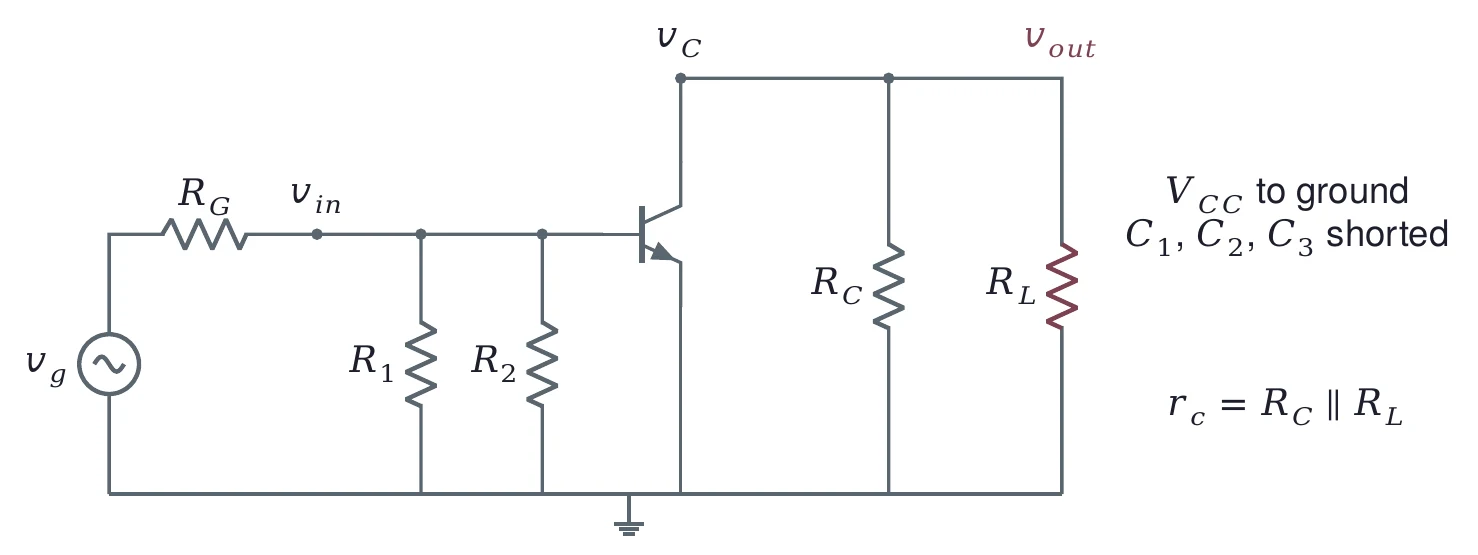
For AC, a DC supply is a short to ground, and so is each large capacitor. and both end up from the base to ground.
One current through two resistances
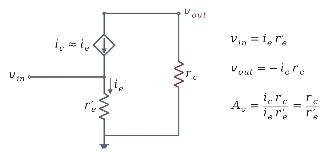
sits across , and almost the same current flows through . The gain is the ratio of the two resistances; the minus sign is the inversion.
r′e is the slope of the junction curve
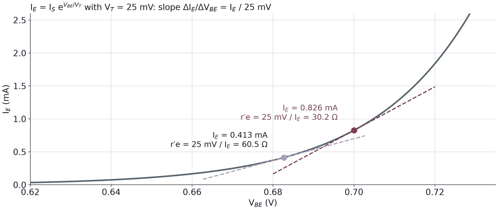
(approx). At = 0.826 mA, = 30.2 Ω. Half the current, twice the .
The voltage gain
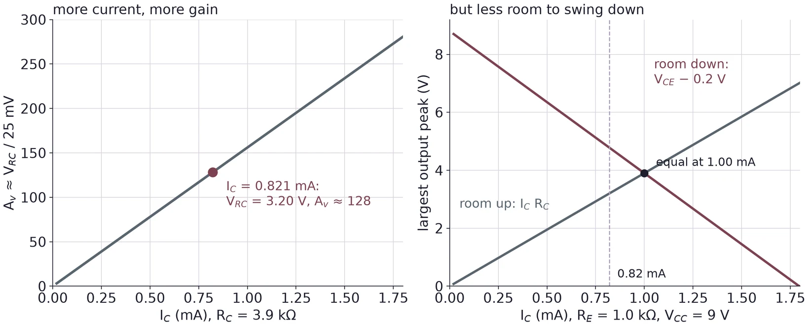
Open load. More raises the gain but eats the room below the Q point.
Without C2 the gain collapses
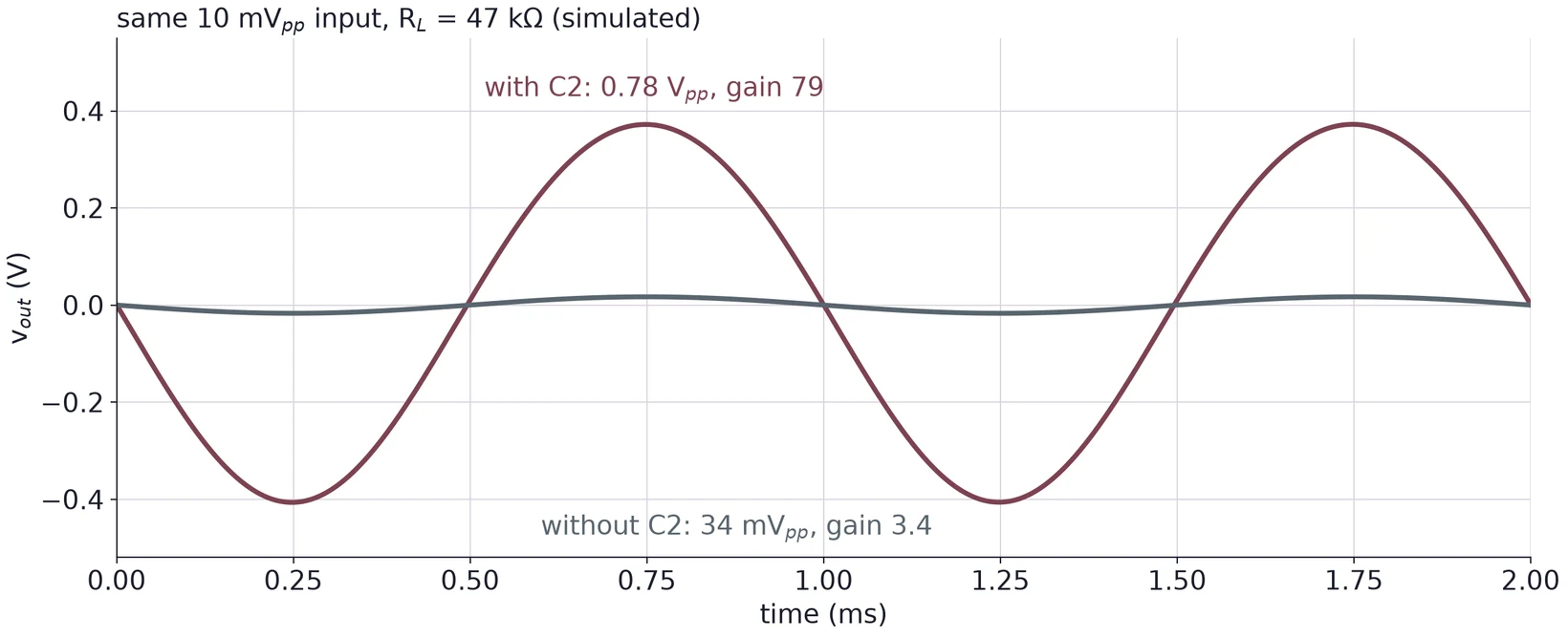
Unbypassed, open load. now takes nearly all of .
The model's r′e is larger than the rule's
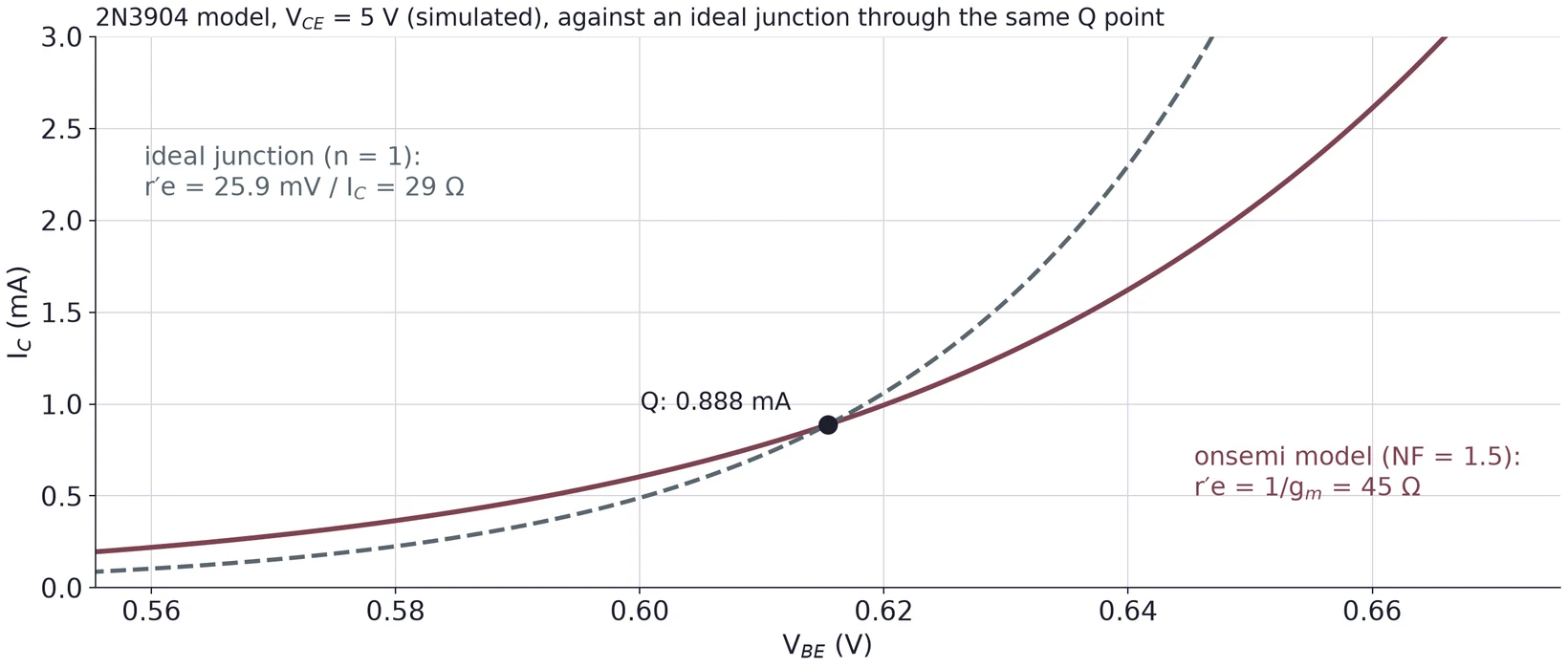
onsemi's model has emission coefficient NF = 1.5, so its is 45 Ω and the simulated gain 79, not 119. Compare your measured gain with both.
Part 4 · Two current gains: first the DC gain
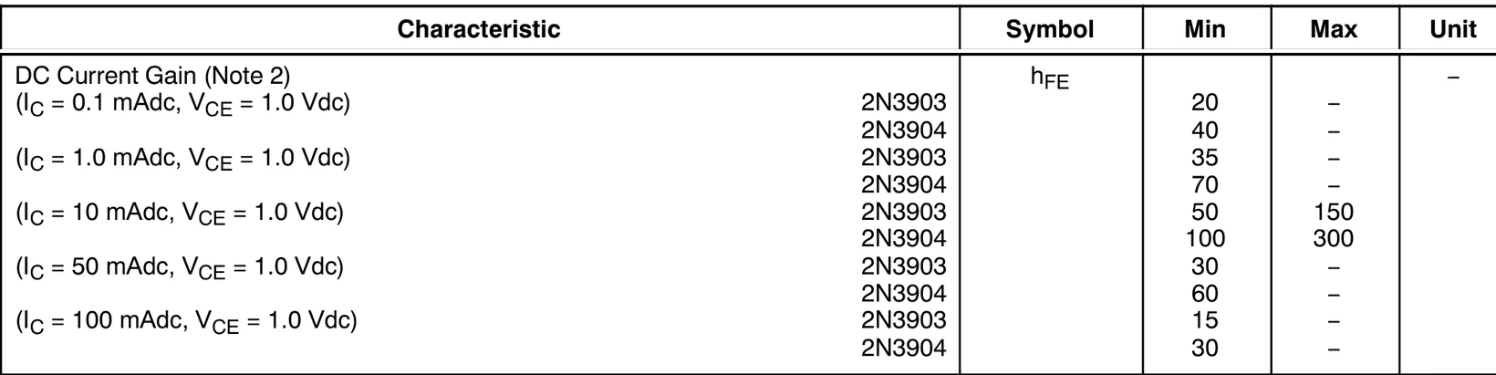
The DC gain sets the bias: at least 70 at 1 mA and 100 to 300 at 10 mA for the 2N3904 (onsemi 2N3903/D, p. 2).
The small-signal gain is a different number
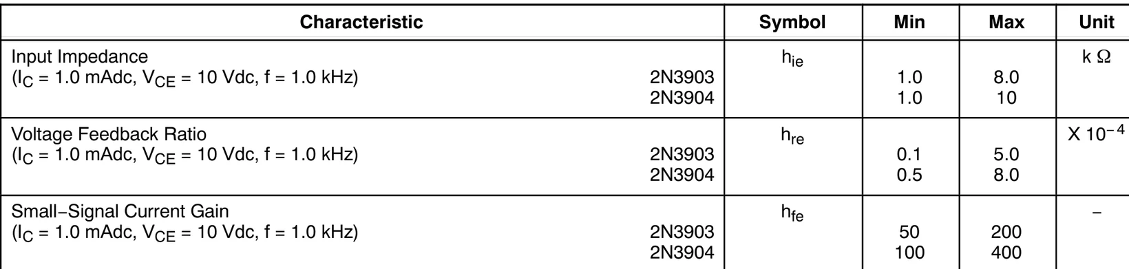
The small-signal gain sets . For the 2N3904, is 100 to 400 at 1 mA, 10 V, 1 kHz (onsemi 2N3903/D, p. 2).
The π model: the base sees βr′e
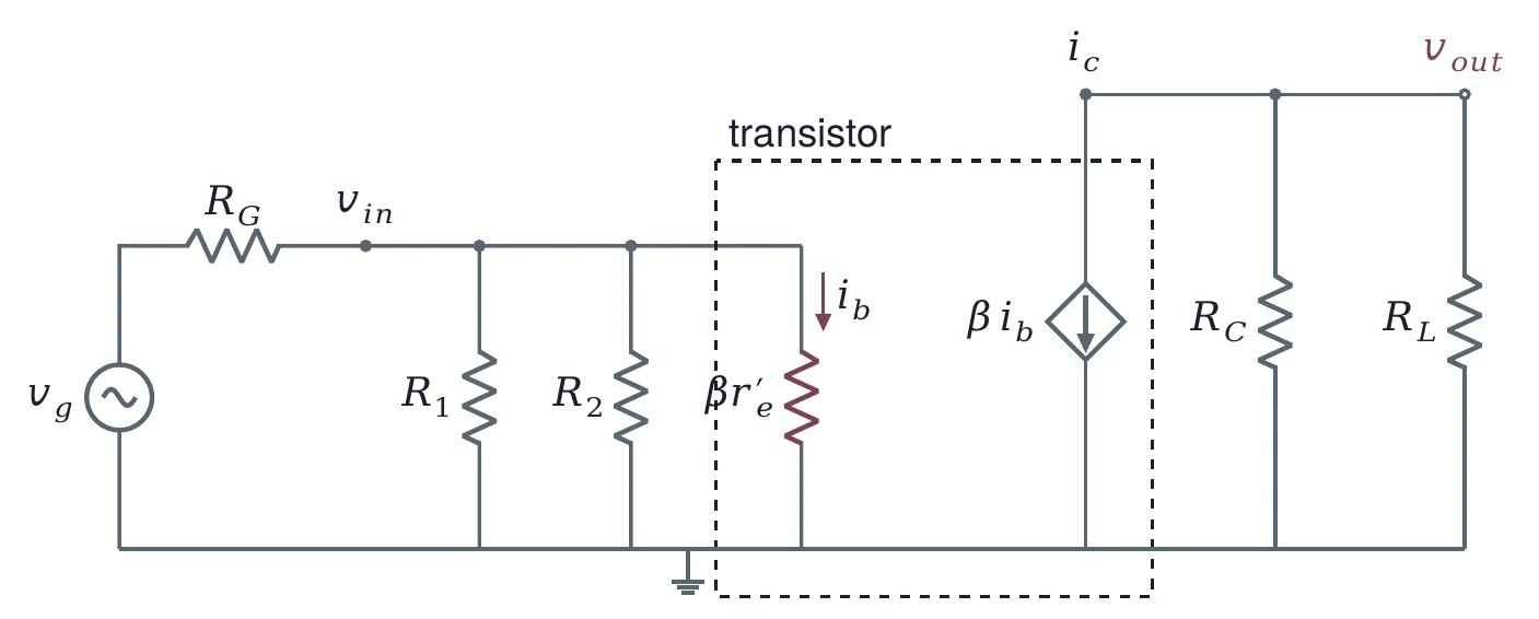
, so the base looks like a resistor = 150 × 30.25 Ω = 4.54 kΩ.
The input impedance of the stage
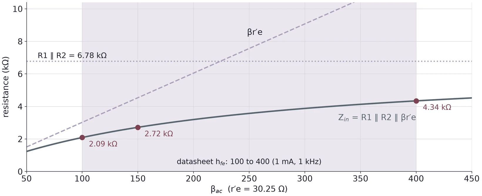
is the smallest of the three, so β sets most of .
The source divides with the input impedance
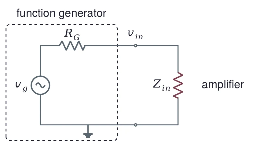
= 50 Ω: 98.2 %, 9.82 mVpp
= 600 Ω: 81.9 %, 8.19 mVpp
= 129 × 9.82 mV = 1.27 Vpp
= 10 mVpp. Measure with the scope at the amplifier's input, not from the generator's setting.
Part 5 · A load sits in parallel with the collector resistor
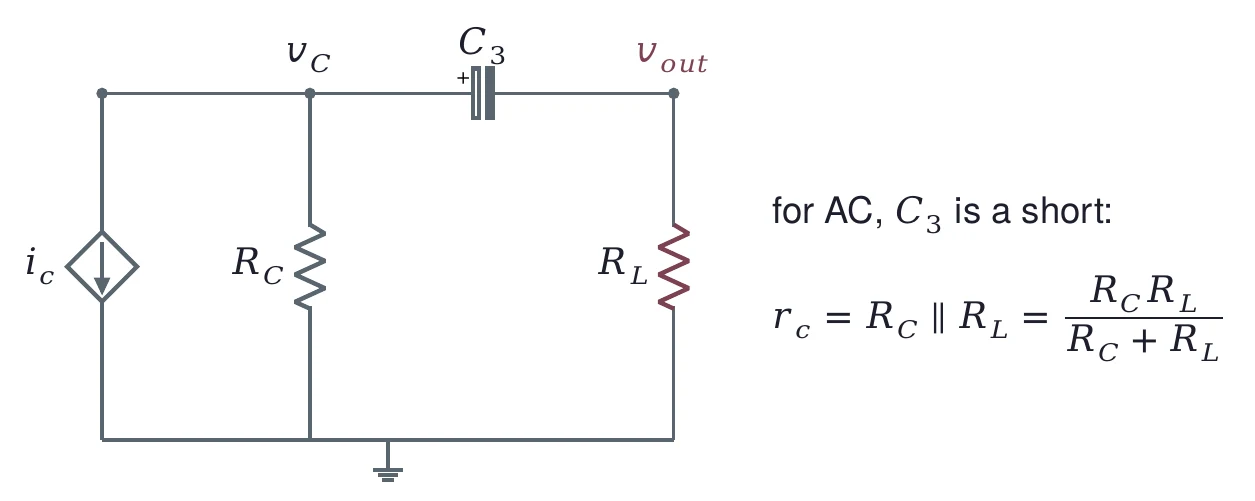
keeps the collector's DC off the load. For AC it is a short, so the load joins and the gain becomes .
Gain falls with the load
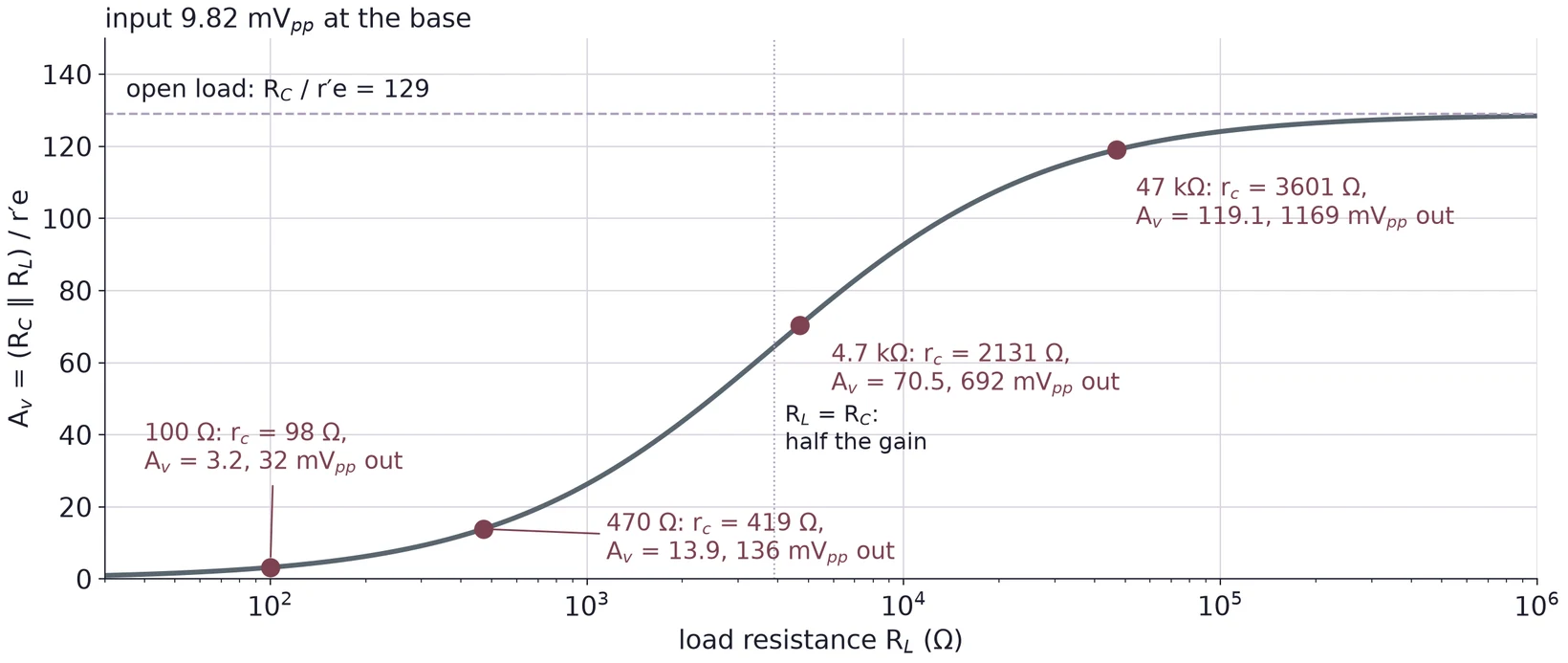
A load equal to halves the gain. A 470 Ω load leaves 13.9.
Swing limits and clipping
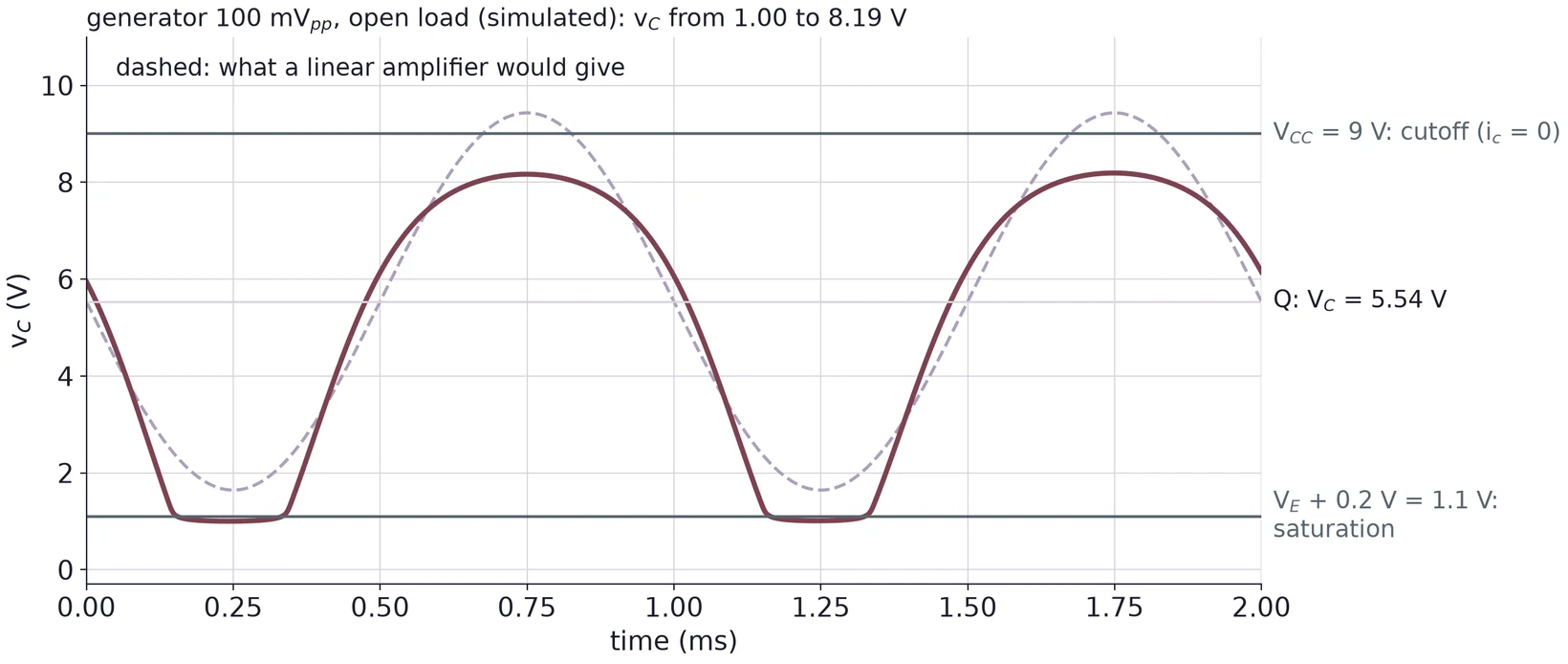
Room up: = 3.20 V. Room down: − 0.2 V = 4.77 V (hand values, β = 150). The smaller one sets the largest clean output.
Keep the input small
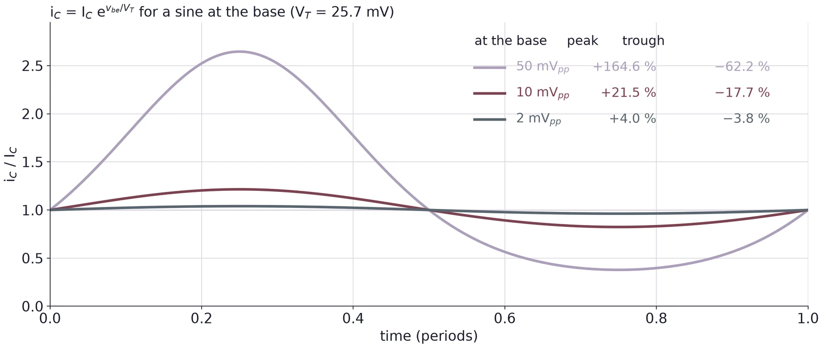
For within 10 %: = 2.5 mV, whatever the bias. Raise the input only while both halves of stay the same height.
Part 6 · Offset, amplitude and phase on the scope
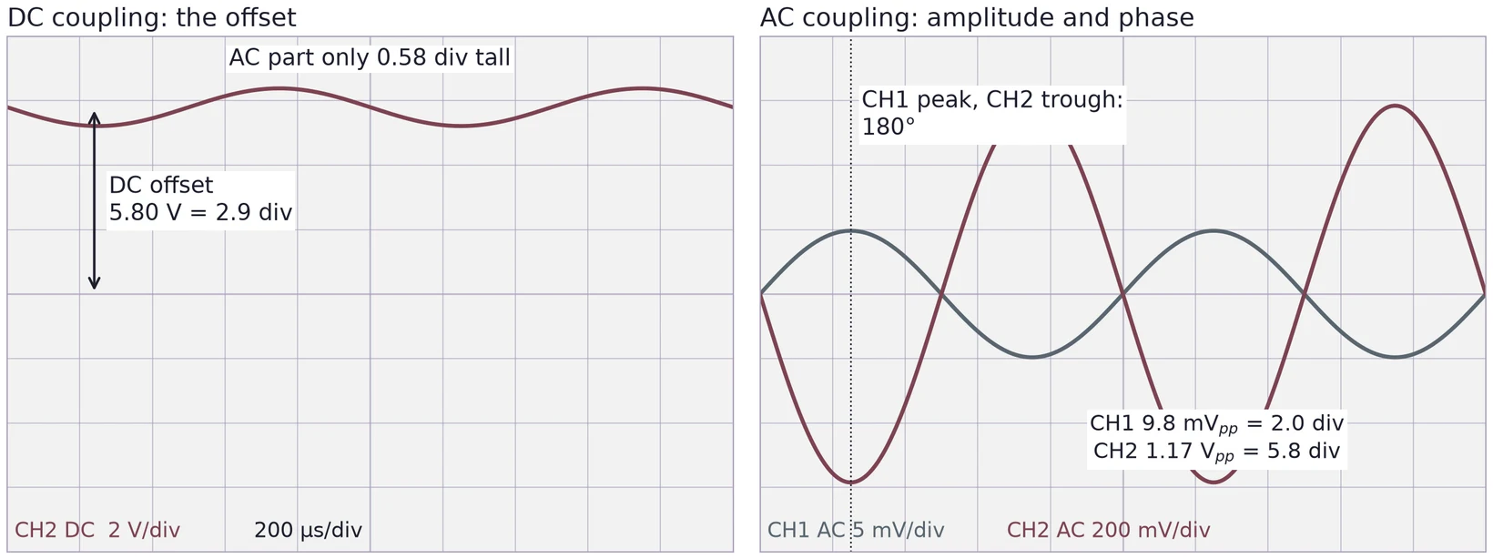
DC coupling shows the offset. AC coupling removes it so you can zoom in on the swing. Drawn from the worked example, not measured.
Three waveforms at once
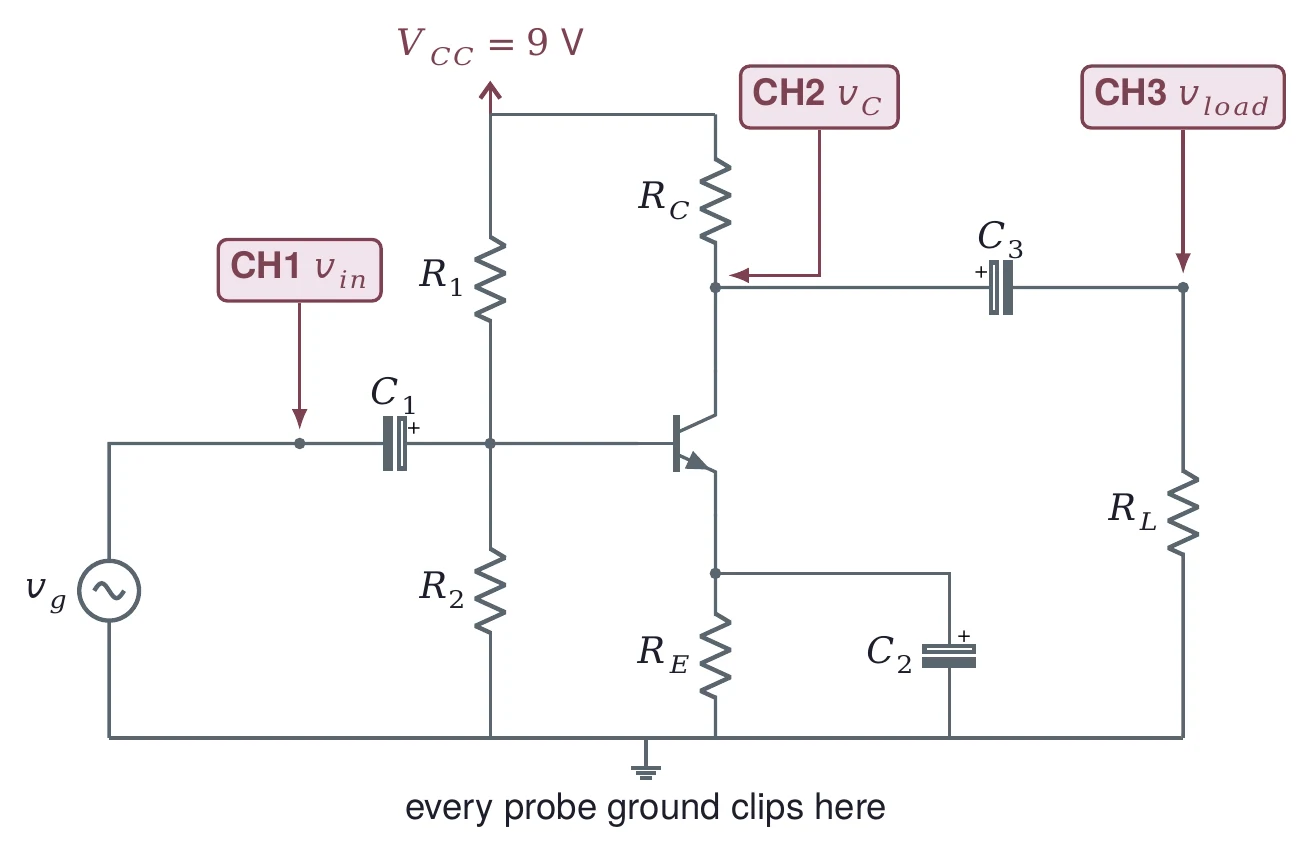
All probe grounds go to one node. Trigger on CH1, and put and on separate scales.
Use ← → to move, Home / End to jump, and F for fullscreen.
Figure descriptions
Slide 2 · Part 1 · Lab 6 in four tasks
Lab 6 in two rows. Bias the transistor: Task 1, DMM pin-to-pin readings of the 2N3904 and 2N3906, then Task 2, divider bias at 5 V: design, measure every current and voltage, find beta dc. Make it amplify: Task 3, a CE amplifier with an input below 50 mVpp at 2 to 20 kHz and an open-load gain above 40, then Task 4, adding C3 and loads of 10 kilohms, 2 kilohms and 300 ohms, with three scope channels at once.
Slide 3 · Task 1 repeats Lab 5's junction check
From the onsemi 2N3903 and 2N3904 datasheet: the NPN symbol with pin numbers, collector 3, base 2 and emitter 1, and drawings of the TO-92 package with straight leads and with bent leads, the leads numbered 1, 2, 3.
Slide 5 · Two divider rules pull apart
Log-log plot of the beta a firm divider needs against the divider-current limit x, where I R1 is below x times I C, for V CC 9 V, V E 0.9 V, V B 1.6 V. The line falls from about 290 at x 0.05 to 14.6 at x 1; at x 0.1 it needs beta above 146. A dashed line marks the datasheet minimum h FE of 70 at 1 mA. A square marks the 39 k and 8.2 k divider at I R1 = 0.23 I C, firm for beta above 68. The region above the line is shaded: both rules met.
Slide 6 · Divider bias holds the Q point when β changes
Two panels. Left: simulated 2N3904 collector curves for base currents of 2 to 12 microamps, I C against V CE from 0 to 9 V, with the DC load line from 1.84 mA at V CE 0 to 9 V at zero current. The hand-calculated Q points for beta 70, 150 and 300 sit almost on top of each other near V CE 5 V and 0.8 mA. Right: I C against beta from 30 to 500. Divider bias stays nearly flat (0.777, 0.821 and 0.842 mA at beta 70, 150, 300), while base bias set for the same current at beta 150 rises in proportion to beta.
Slide 7 · Part 2 · A capacitor passes AC and blocks DC
Log-log plot of capacitive reactance X C equals 1 over 2 pi f C against frequency from 10 Hz to 100 kHz for 1, 10 and 100 microfarads: three parallel falling lines. At 1 kHz they read 159, 15.9 and 1.59 ohms. A note says low f gives large X C (an open circuit at DC) and high f gives small X C (a short for AC).
Slide 8 · The coupling capacitor is a high-pass filter
A source v in drives a series capacitor C into a resistor R to ground; v out is taken across R. Notes: at high f, X C is small and v out is about v in; at DC, X C is open and v out is 0.
Slide 9 · The bypass capacitor grounds the emitter for AC
Two circuits. Left: a source v in, a series resistor R, and a capacitor C from the output to ground: at high frequency C shorts v out to ground. Right: a transistor emitter with R E to ground and the electrolytic capacitor C2 across it: for AC, v E is held at its DC value.
Slide 11 · Electrolytics: + goes to the higher DC side
A purple radial aluminium electrolytic capacitor marked 50 V, 100 microfarads, with a light stripe of minus signs along one side marking the negative lead.
Slide 12 · Part 3 · The common-emitter amplifier
The common-emitter amplifier. A generator v g of 10 mVpp at 1 kHz with R G 50 ohms feeds v in, then C1 10 microfarads into the base node v B. The divider R1 39 kilohms from V CC 9 V and R2 8.2 kilohms to ground biases the base of a 2N3904. R C 3.9 kilohms runs from V CC to the collector v C; R E 1.0 kilohm runs from the emitter v E to ground, bypassed by C2 470 microfarads. C3 10 microfarads couples the collector to the load R L 47 kilohms at v out. The electrolytic capacitors have their plus side toward the base, the emitter and the collector.
Slide 13 · DC plus AC at every node
Simulated waveforms over two periods at five nodes, stacked. v in: 9.85 mVpp around 0 V. v B: the same 9.85 mVpp riding on 1.51 V DC. v E: flat at 0.90 V, no AC. v C: 0.78 Vpp around 5.54 V, upside down relative to v B. v out: the same 0.78 Vpp centered on 0 V.
Slide 14 · The output is inverted
Simulated v in (left axis, millivolts) and v out (right axis, volts) over two periods: when v in reaches its peak, v out is at its trough. v in 9.85 mVpp, v out 0.78 Vpp with R L 47 kilohms, shifted 179 degrees.
Slide 15 · The AC equivalent circuit
The AC equivalent circuit: v g with R G drives v in at the base. R1 and R2 both go from the base to ground. The emitter goes straight to ground. The collector v C connects R C and R L, both to ground, and v out. Notes: V CC to ground, C1, C2 and C3 shorted; r c equals R C in parallel with R L.
Slide 16 · One current through two resistances
The T model of the transistor: v in drives the top of r prime e, which goes to ground and carries i e. A current source i c, about equal to i e, flows from the output node down into the same point. The output node v out connects to r c to ground. Equations: v in = i e r prime e, v out = minus i c r c, A v = i c r c over i e r prime e = r c over r prime e.
Slide 17 · r′e is the slope of the junction curve
The exponential junction curve I E = I S e to the V BE over V T with V T 25 mV, from 0.62 to 0.735 V. Two dashed tangents: at 0.826 mA the slope gives r prime e = 25 mV over I E = 30.2 ohms; at 0.413 mA it gives 60.5 ohms, a flatter tangent.
Slide 18 · The voltage gain
Two panels against collector current from 0 to 1.8 mA. Left: A v approximately V RC over 25 mV, a straight line with R C 3.9 kilohms; the point at I C 0.821 mA has V RC 3.20 V and A v about 128. Right: the largest output peak. Room up, I C R C, rises; room down, V CE minus 0.2 V with R E 1.0 kilohm and V CC 9 V, falls. They are equal at 1.00 mA; a dashed line marks 0.82 mA.
Slide 19 · Without C2 the gain collapses
Simulated v out for the same 10 mVpp input with R L 47 kilohms: with C2 the output is 0.78 Vpp, a gain of 79; without C2 it is 34 mVpp, a gain of 3.4.
Slide 20 · The model's r′e is larger than the rule's
Simulated I C against V BE for the onsemi 2N3904 model at V CE 5 V, and the curve of an ideal junction (emission coefficient 1) through the same Q point at 0.888 mA. The ideal curve is steeper: r prime e = 25.9 mV over I C = 29 ohms. The model, with NF 1.5, gives r prime e = 1 over g m = 45 ohms.
Slide 21 · Part 4 · Two current gains: first the DC gain
DC current gain rows from the onsemi 2N3903 and 2N3904 datasheet, at V_CE = 1.0 V. For the 2N3904, hFE is at least 40 at 0.1 mA, 70 at 1.0 mA, 100 to 300 at 10 mA, 60 at 50 mA and 30 at 100 mA; the 2N3903 rows are lower.
Slide 22 · The small-signal gain is a different number
Small-signal rows of the onsemi 2N3903 and 2N3904 datasheet, measured at I_C = 1.0 mA, V_CE = 10 V and 1.0 kHz, under the table header. Input impedance h_ie: 1.0 to 8.0 kilohms for the 2N3903 and 1.0 to 10 kilohms for the 2N3904. Voltage feedback ratio h_re: 0.1 to 5.0 and 0.5 to 8.0 times 10 to the minus 4. Small-signal current gain h_fe: 50 to 200 for the 2N3903 and 100 to 400 for the 2N3904.
Slide 23 · The π model: the base sees βr′e
The pi model of the stage, redrawn from the handwritten notes with the base resistor labeled beta r prime e. v g and R G drive v in. R1, R2 and beta r prime e, which carries i b, go from the input node to ground. Inside a dashed transistor box, a current source beta i b, labeled i c, flows from the output node to ground. R C and R L also go from the output node to ground; v out is at the top.
Slide 24 · The input impedance of the stage
Resistance in kilohms against beta ac from 50 to 450, with r prime e 30.25 ohms. Dashed: beta r prime e, a rising line. Dotted: R1 parallel R2 = 6.78 kilohms. Solid: Z in = R1 parallel R2 parallel beta r prime e, which rises slowly: 2.09 kilohms at beta 100, 2.72 at 150, 4.34 at 400. The datasheet h fe range of 100 to 400 is shaded.
Slide 25 · The source divides with the input impedance
A function generator drawn as v g behind R G inside a dashed box, connected at v in to the amplifier's input impedance Z in to ground.
Slide 26 · Part 5 · A load sits in parallel with the collector resistor
The output side for AC: a current source i c from v C to ground, R C from v C to ground, then C3 in series to v out and R L to ground. For AC, C3 is a short, so r c = R C parallel R L = R C R L over R C plus R L.
Slide 27 · Gain falls with the load
A v = R C parallel R L over r prime e against load resistance from 30 ohms to 1 megohm on a log axis, rising to the open-load value of 129. Points: 47 kilohms, r c 3601 ohms, A v 119.1, 1169 mVpp out; 4.7 kilohms, 2131 ohms, 70.5, 692 mVpp; 470 ohms, 419 ohms, 13.9, 136 mVpp; 100 ohms, 98 ohms, 3.2, 32 mVpp. Input 9.82 mVpp at the base. A dotted line at R L = R C marks half the gain.
Slide 28 · Swing limits and clipping
Simulated v C for a 100 mVpp generator signal with open load, over two periods. The output runs from 1.00 to 8.19 V around the Q point of 5.54 V. Its bottom is flat at about 1.0 V, near the V E plus 0.2 V = 1.1 V line, where the transistor saturates; its top is rounded and stays below the 9 V cutoff line. A dashed sine shows what a linear amplifier would give: from 1.64 to 9.43 V, past the 9 V line.
Slide 29 · Keep the input small
i C over I C during one period of a sine at the base, from i C = I C e to the v be over V T with V T 25.7 mV. 2 mVpp: plus 4.0 and minus 3.8 percent, almost symmetric. 10 mVpp: plus 21.5 and minus 17.7 percent. 50 mVpp: plus 164.6 and minus 62.2 percent, a tall peak and a shallow trough.
Slide 30 · Part 6 · Offset, amplitude and phase on the scope
Two scope screens drawn from the worked example. Left, DC coupling at 2 V per division and 200 microseconds per division: v C sits 5.80 V, 2.9 divisions, above the center line, and its AC part is only 0.58 divisions tall. Right, AC coupling: CH1 at 5 mV per division shows 9.8 mVpp, 2.0 divisions; CH2 at 200 mV per division shows 1.17 Vpp, 5.8 divisions. Where CH1 peaks, CH2 is at a trough: 180 degrees.
Slide 31 · Three waveforms at once
The CE amplifier with three scope probes: CH1 on v in at the generator side of C1, CH2 on v C at the collector, and CH3 on v load across R L after C3. Every probe ground clips to the circuit ground.