1 Where Lab 2 Sits
Lab 1 converted between voltage, current and light, and every op-amp stage in it was linear. Lab 2 adds the first nonlinear operation: multiplication. The AD633 takes two voltages and returns their product, and that single operation does three very different jobs. It moves a signal to a new frequency (a mixer), it squares a voltage, and, placed inside a feedback loop, it takes a square root.
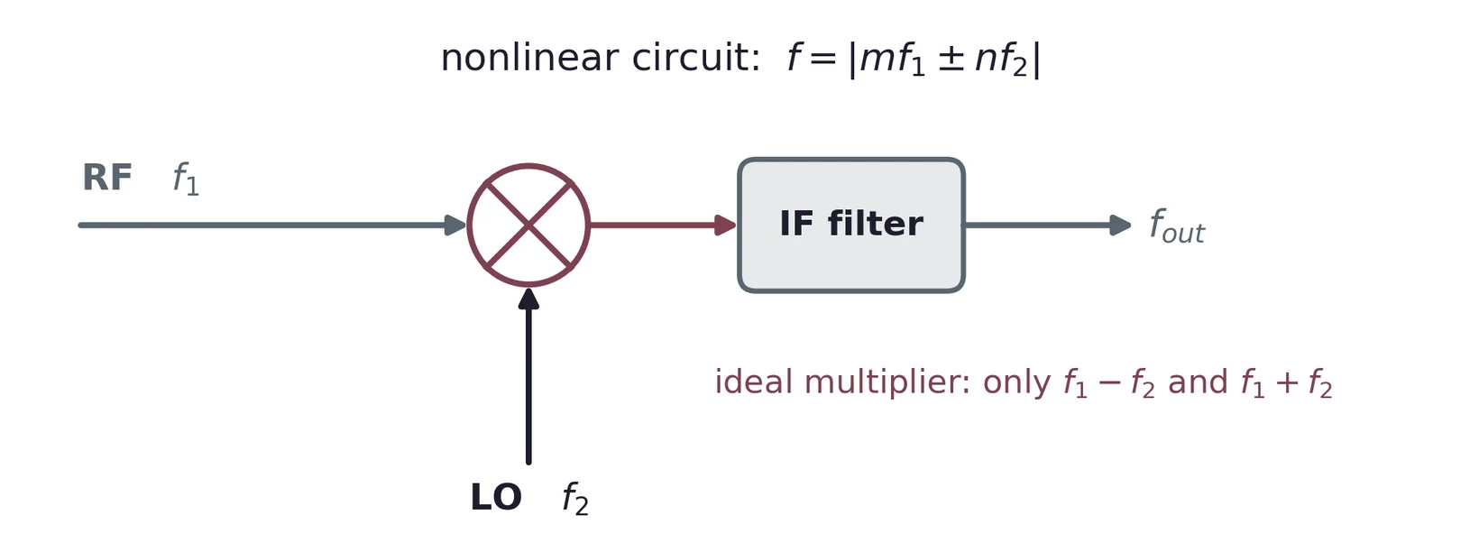
Multiplication moves information in frequency: the product of two tones is a pair of tones at their sum and difference. The same multiplier, with both inputs tied together, squares. And put a function in the feedback path of a high-gain amplifier, and the loop computes its inverse, provided the function only rises (or only falls) over the range you use. Lab 2 uses all three facts.
1.1 Task map
| Lab 2 task | What you do | Concept & section |
|---|---|---|
| 1 | Wire the AD633 with 0.1 µF decoupling; square an input; measure many points; quadratic fit in Python | The AD633; decoupling; squaring; fitting (§6, §7) |
| 2 | Consider offset, scale-factor and nonlinearity errors; design and build an offset trim from the datasheet | Error signatures; the trim network (§8) |
| 3 | Offsets under ±50 mV; squarer in a feedback loop for a square root; measure; square-root fit | Inverting a function with feedback (§9) |
Sections 2–5 explain mixing, the best-known use of a multiplier and the "mixing" in the lab's title. The lab itself uses the AD633 at low frequency, as a squarer and then as a square-rooter.
2 What a Multiplier Does
2.1 One line of algebra
Multiply two cosines, and . Write each with Euler's formula, , multiply out the four exponentials, and pair them back into cosines:
The four products are and , and each ± pair is twice a cosine:
with . A difference tone at and a sum tone at . The input frequencies themselves are gone. The phases subtract and add too, which matters in §2.3.
2.2 In time and in frequency
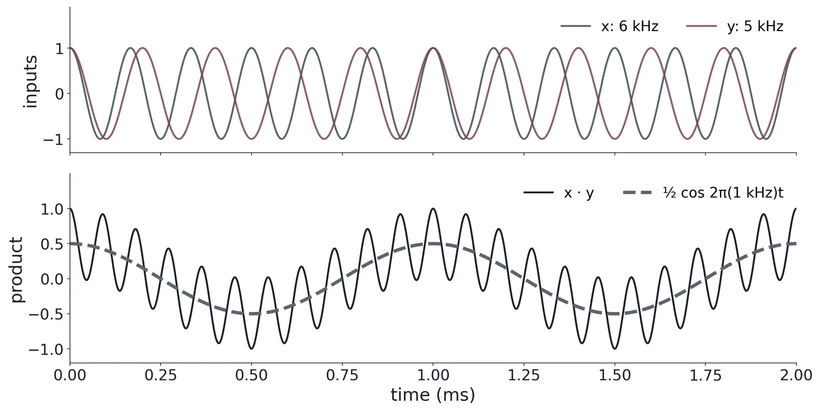
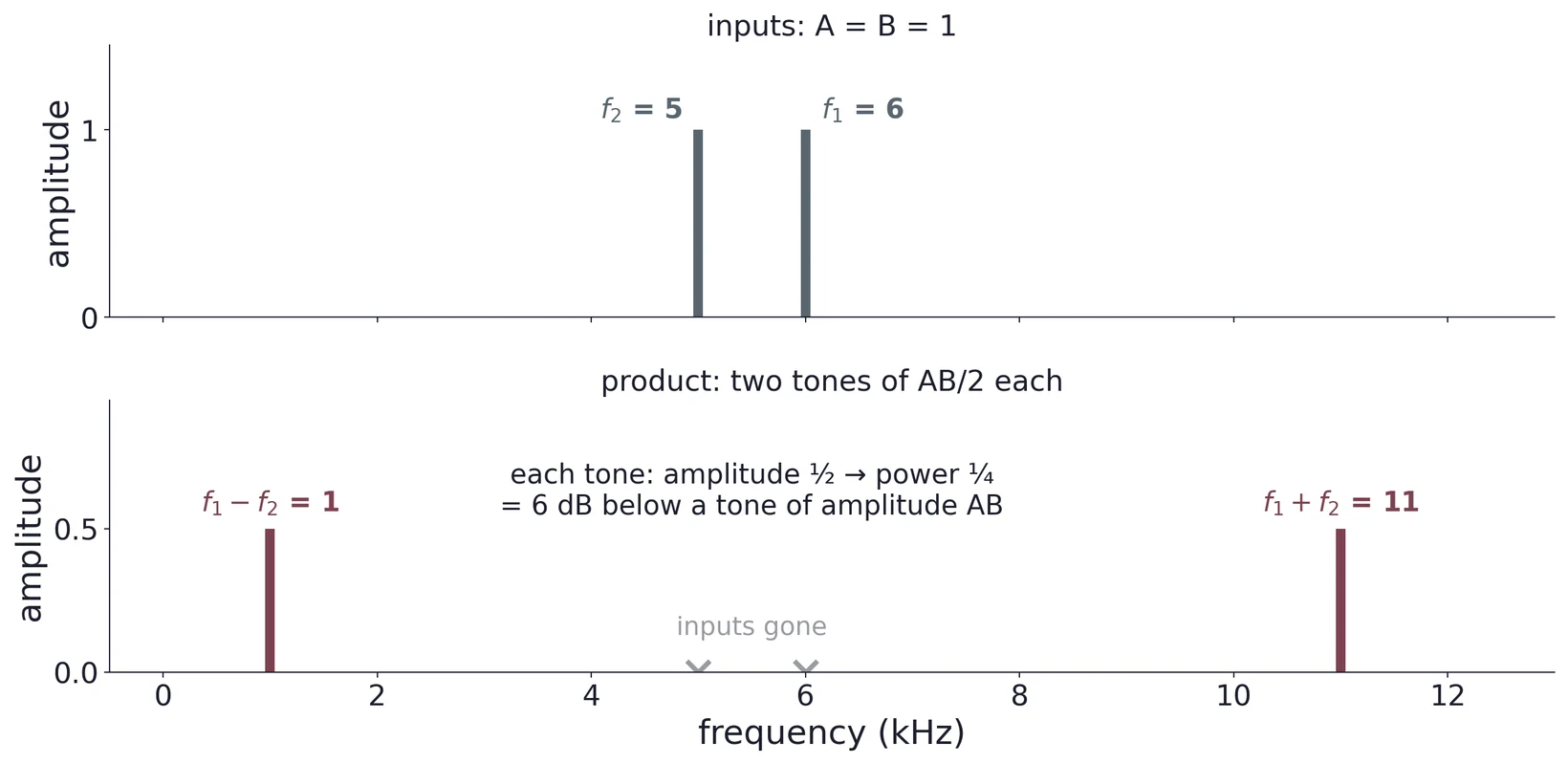
A filter after the multiplier keeps whichever term is wanted: a low-pass keeps 1 kHz, a band-pass at 11 kHz keeps the sum. The two products are apart (10 kHz here, with the lower input frequency), far more than the 1 kHz between the inputs, so the filter is easy to build.
2.3 Amplitude, power and the 6 dB
For inputs and , each output tone has amplitude . Power in a resistor goes as , so each tone carries of the power of a tone of amplitude : 6 dB down. With the LO amplitude normalized to one, the kept tone has half the RF amplitude. That is the 6 dB conversion loss of an ideal multiplying mixer, and it is why a mixer is normally followed by gain.
Where do the 6 dB go? Half of it, 3 dB, goes in the multiplication itself: the LO cosine spends much of each cycle near zero, and its mean square is only ½. The other 3 dB goes at the filter: what is left is shared equally between the sum and the difference tones, and you keep only one of them.
A real multiplier has a scale factor in V⁻¹ (the AD633's is 1/10 V), so each tone is volts. The phase term is useful as well: with equal frequencies, the difference term is a DC voltage , so a multiplier followed by a low-pass filter measures phase. That is the phase detector at the heart of lock-in amplifiers and phase-locked loops.
(a) Find the output frequencies when 12.0 kHz and 10.7 kHz are multiplied. Which circuit element selects the one you want?
(b) Both inputs are 3 V amplitude into an AD633. What is the amplitude of each output tone?
(c) Set in Equation (2). What are the two output terms, and what does the first one represent? (This is the squaring case, §7.)
3 Any Nonlinear Circuit Mixes
A multiplier is the cleanest mixer, but any nonlinearity mixes. Expand a diode's exponential law in a Taylor series about its bias point,
and put in two tones, . The term contains : exactly the product of §2, with its sum and difference tones, plus DC and , . The term adds , and terms, and so on. In general a nonlinear circuit produces every
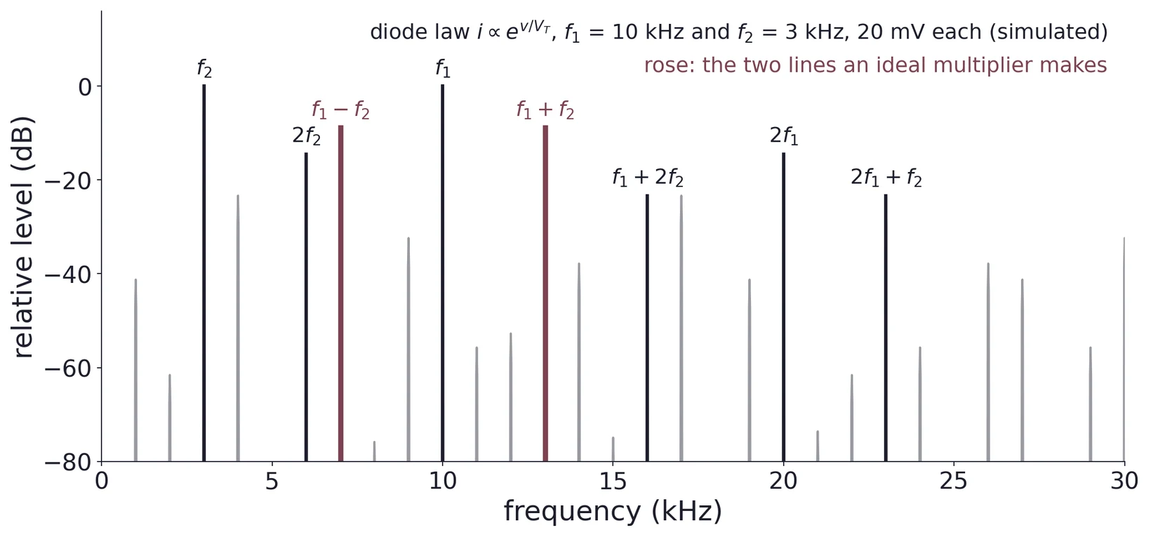
A practical mixer therefore depends on its frequency plan and output filter to keep one product and reject the rest. The AD633's advantage is that it is built to multiply and nothing else, so its unwanted products are small (§6.4).
4 The Radio Receiver
4.1 The superheterodyne
Most radio receivers are superheterodynes. A superhet shifts the station you tune to down to one fixed intermediate frequency (IF), and does most of its filtering and amplification there.
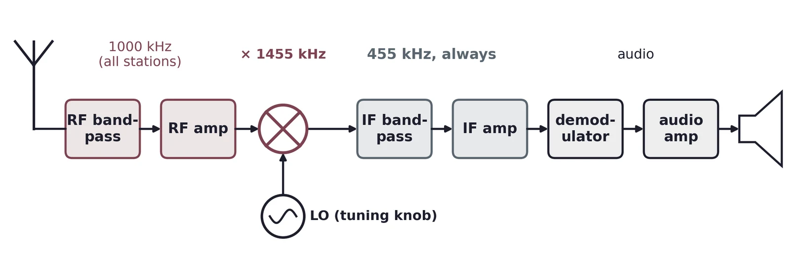
- Antenna. Every station arrives at once, at the microvolt level.
- RF filter and amplifier. A broad band-pass around the wanted band, plus gain; it also rejects the image (§4.3).
- Local oscillator. A tunable sine wave. Tuning the radio is setting .
- Mixer. Multiplies RF by the LO; the difference is kept.
- IF filter and amplifier. A sharp band-pass at the fixed IF does almost all of the selectivity and gain, because a sharp filter is easy to build well at one frequency. Broadcast AM uses 455 kHz; broadcast FM uses 10.7 MHz.
- Demodulator and audio amplifier. Recover the message and drive the speaker.
4.2 Choosing the local oscillator
The kept difference must equal the IF:
For a wanted station there are two solutions: (high-side injection) or (low-side). Broadcast AM receivers use high-side injection because the oscillator then tunes over a much smaller frequency ratio. For the 540–1700 kHz band, a high-side LO runs from 995 to 2155 kHz, a ratio of about 2.2. A low-side LO would have to run from 85 to 1245 kHz, a ratio of almost 15, which is much harder to build.
4.3 The image frequency
The mixer sees only , so it cannot tell a signal above the oscillator from one the same distance below it. A second input, the image, also lands on the IF, on the opposite side of the LO from the wanted station and away from it.
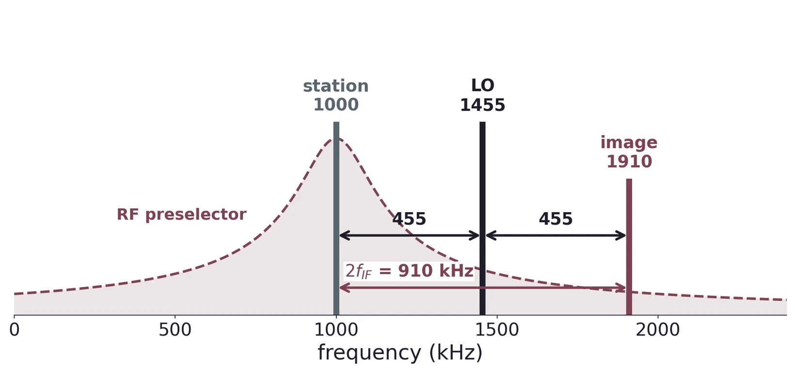
- High-side: = 1000 + 455 = 1455 kHz. The image is at = 1910 kHz, since |1910 − 1455| = 455.
- Low-side: = 1000 − 455 = 545 kHz. The image is at = 90 kHz, since |90 − 545| = 455.
Either way the image is = 910 kHz from the station. A higher IF moves the image further away and makes the preselector's job easier, one reason FM uses 10.7 MHz.
4.4 AM and FM ride along
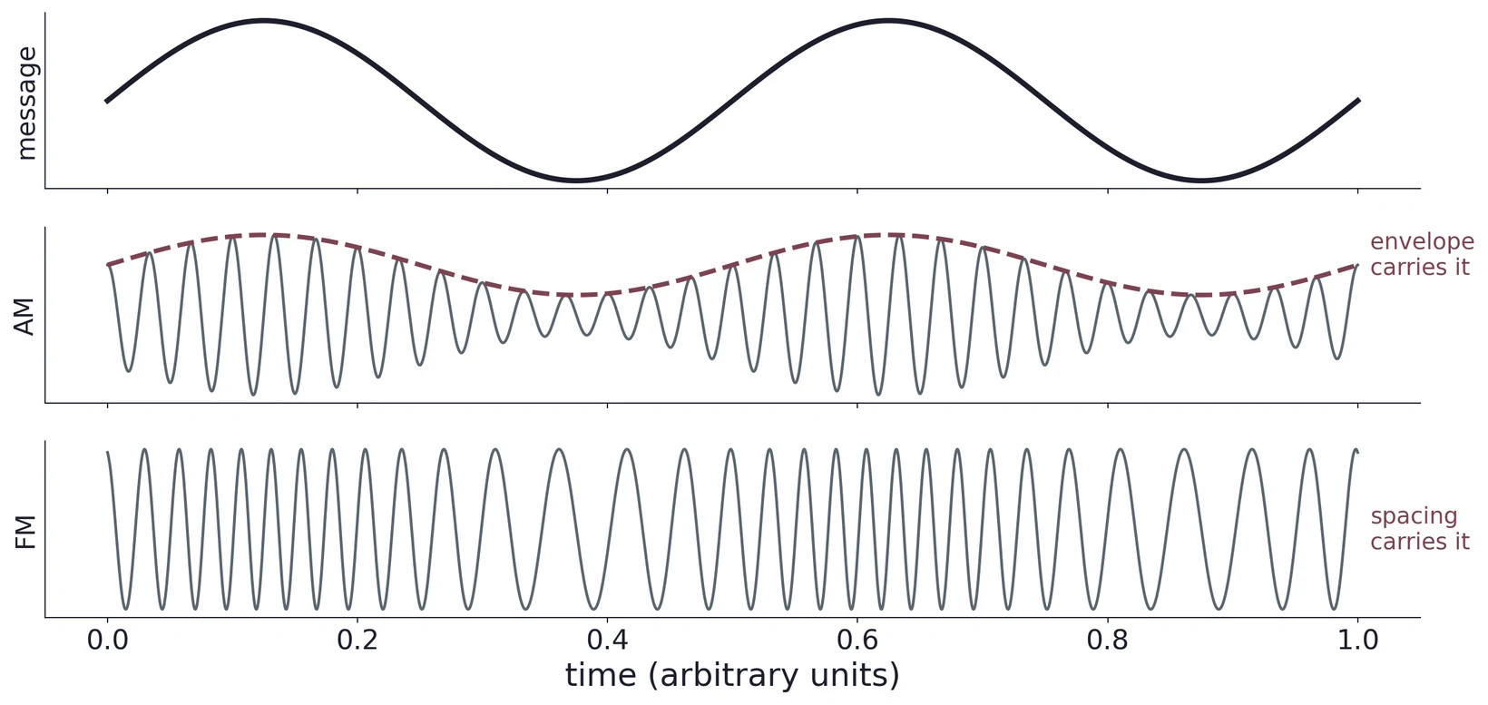
Mixing does not care whether the signal is AM or FM. Shifting a carrier in frequency keeps its envelope (the AM) and its frequency swings (the FM), so the RF, LO, mixer and IF stages are the same for both. They part ways only at the demodulator: an envelope detector for AM, a frequency discriminator or phase-locked loop for FM. Because an FM signal's amplitude carries no information, the receiver can clip it flat with a limiter, which strips off most amplitude noise. That is a large part of why FM sounds cleaner than AM.
(a) A receiver with = 455 kHz is tuned to 1200 kHz with high-side injection. Find and the image frequency.
(b) Repeat for an FM receiver with = 10.7 MHz tuned to 99.3 MHz. Is the image inside the 88–108 MHz band, and why does that matter?
(c) A designer proposes a 100 kHz IF for sharper filtering. What does it cost, quantitatively, in image separation?
5 The NE602: a Mixer on a Chip
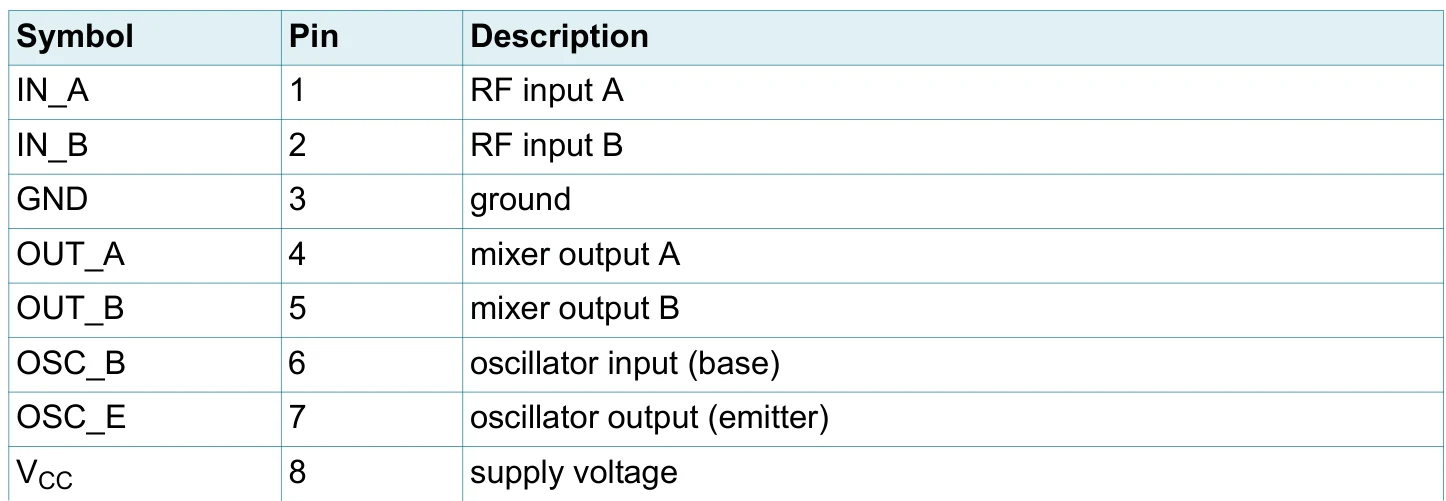
The NE602, now sold as the NXP SA602A, packages an oscillator and a double-balanced mixer in one 8-pin IC. It is the front end of countless shortwave, amateur and communications receivers.
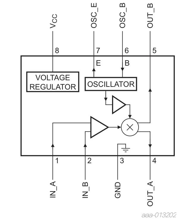
5.1 Inside: a Gilbert cell
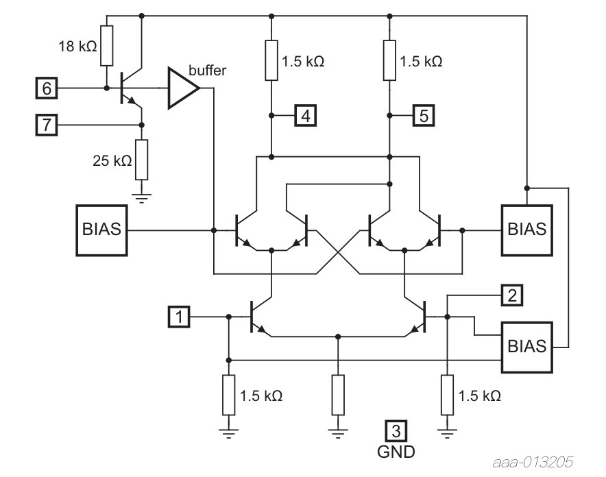
The lower pair turns the RF voltage into a pair of currents whose difference is proportional to the RF signal. The oscillator switches the upper pairs so that this difference current is routed to one output or the other on alternate half cycles: the output current is the RF signal times ±1 at the LO rate. A square wave at contains , , …, so the output contains plus weaker products at the odd harmonics. Because the cell is balanced, the RF and LO themselves largely cancel at the output: "double-balanced".
Its blocks are worth knowing, because they reappear in every receiver front end:
- Local oscillator. An internal oscillator transistor on pins 6 and 7, with an external crystal or tuned circuit, or an external LO signal.
- Differential signal ports. The RF inputs and mixer outputs are differential, so coupling, biasing and the termination of unused inputs all matter; the inputs are biased internally, so couple signals in through a capacitor or transformer and never apply a DC bias from outside.
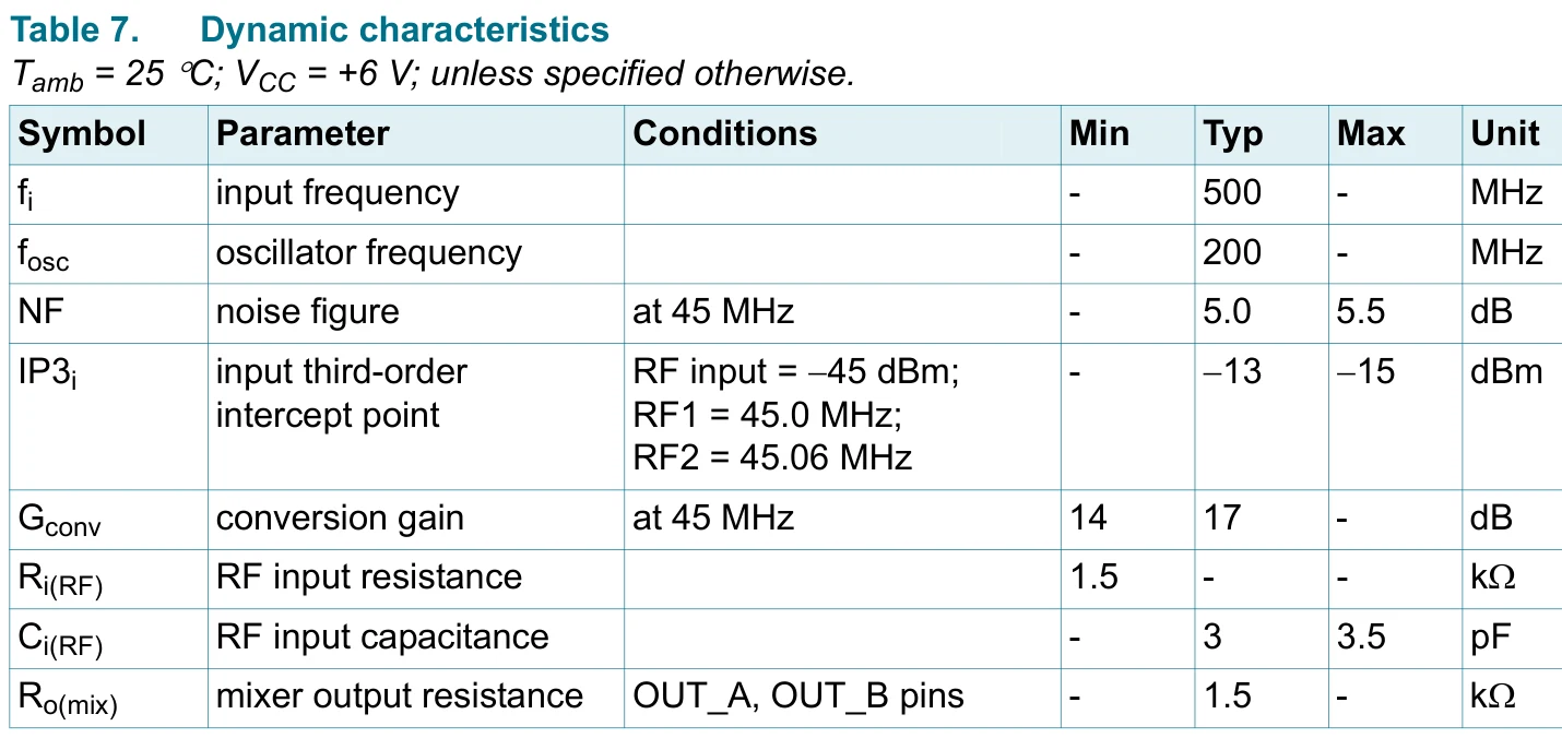
- Nonlinear mixer core. The Gilbert cell. It has 17 dB of conversion gain, where the ideal multiplier of §2.3 loses 6 dB.
- Output network. External tuned circuits select the wanted IF.
- Supply decoupling. A bypass capacitor at pin 8 keeps supply noise and oscillator currents out of the signal path.
6 The AD633 Analog Multiplier
6.1 Inside and transfer equation
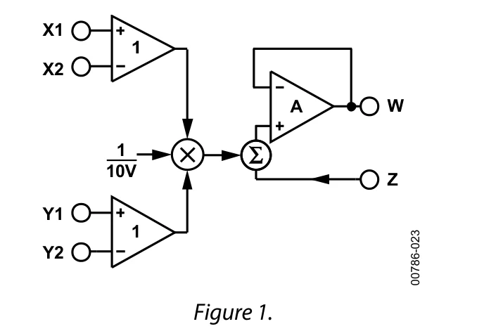
The AD633 is a four-quadrant multiplier: both inputs may take either polarity and the output sign comes out right in all four combinations. Inside, the X and Y voltages are converted to currents and multiplied in a translinear core; a buried Zener reference sets the 10 V scale; the output amplifier adds after the product. Two features of Equation (6) matter for every Lab 2 measurement. The inputs are differential, so the unused input of each pair must be tied to a defined potential, normally ground, and never left floating. And the 10 V divisor keeps the output within its ±11 V range for inputs up to ±10 V.
6.2 Pinout and wiring
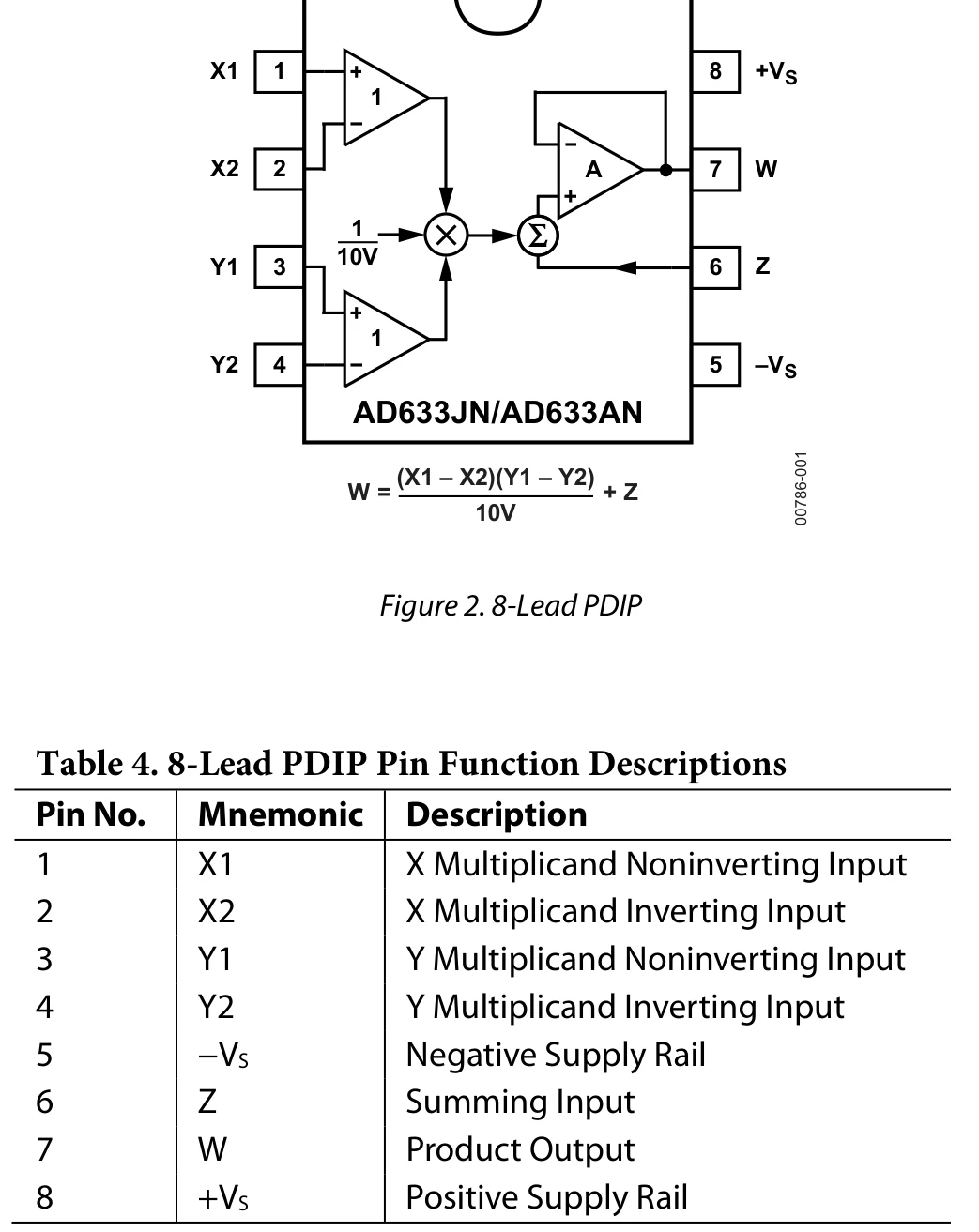
The SOIC package (AD633JR/AR) uses a different arrangement: pin 1 is Y1 there. Check the part number against the datasheet before wiring; putting a supply on a signal pin can destroy the chip.
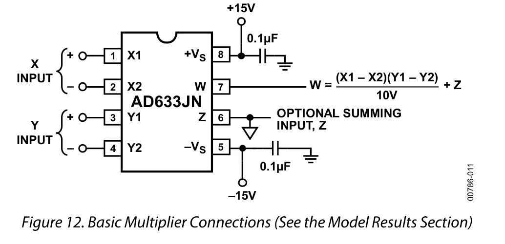
6.3 Decoupling
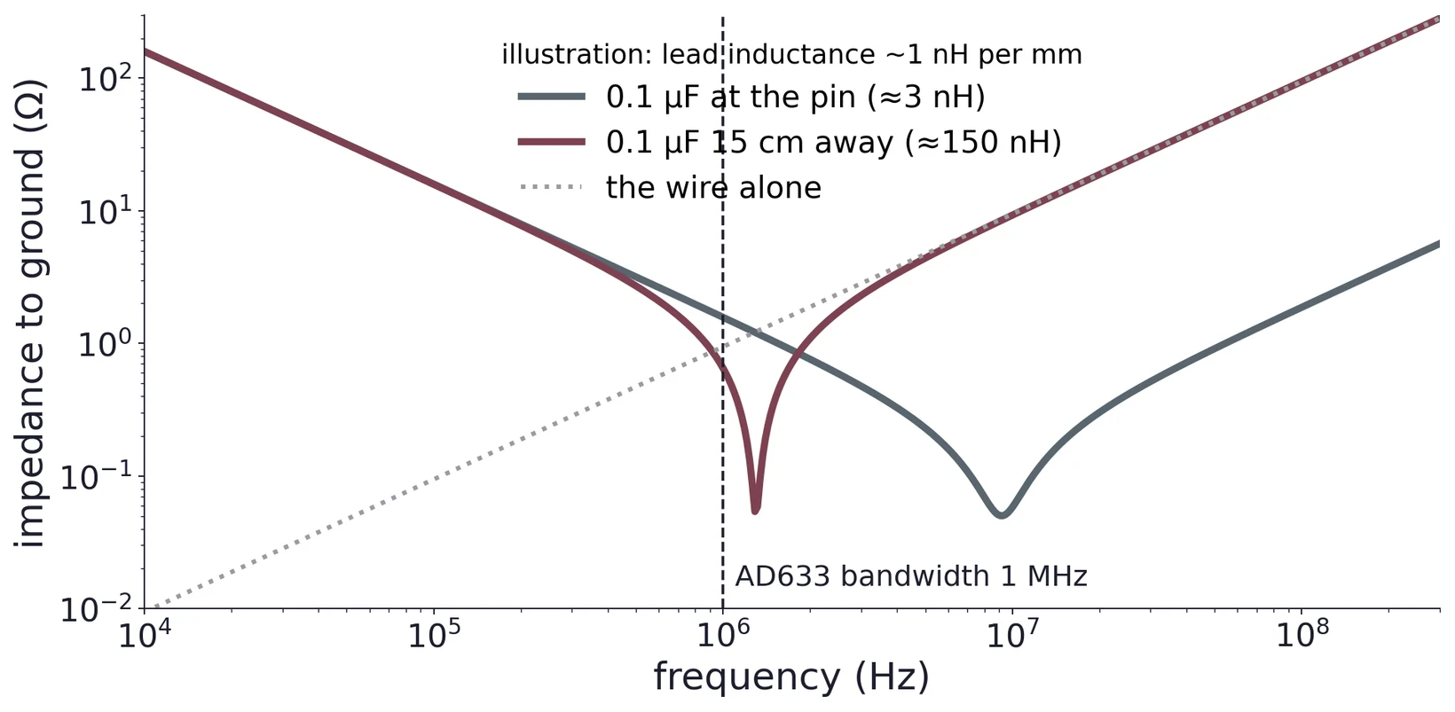
A capacitor is a short to ground only below its self-resonance, , where includes every millimetre of lead and breadboard strip (roughly 1 nH per mm). A long connection moves the resonance down into the AD633's 1 MHz bandwidth, exactly where the chip still has gain.
Task 1 asks for about 0.1 µF on each supply rail. Place each capacitor at its supply pin, not across the breadboard. Without it the multiplier can oscillate, which shows up as a fuzzy output trace and ruins the accuracy measurements that follow.
6.4 What the datasheet promises
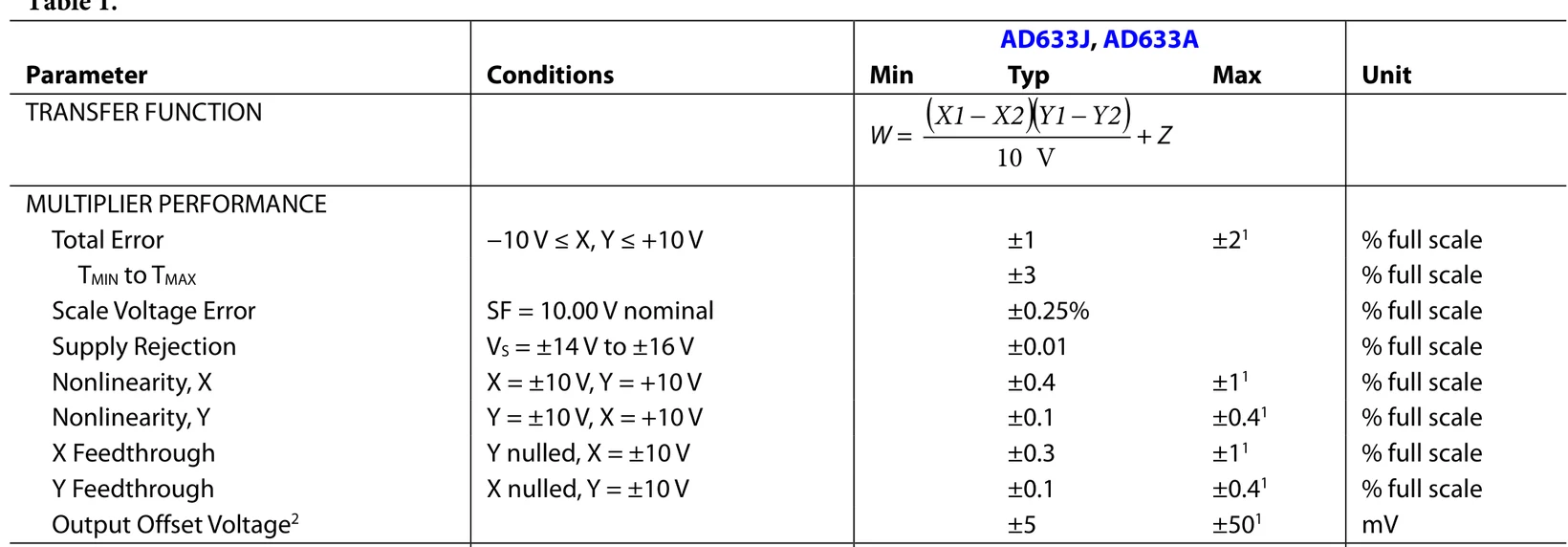
"Full scale" is 10 V, so ±2 % is ±200 mV at worst. The same table gives the input offset, ±5 mV typ and ±30 mV max, a 1 MHz small-signal bandwidth and a 20 V/µs slew rate.
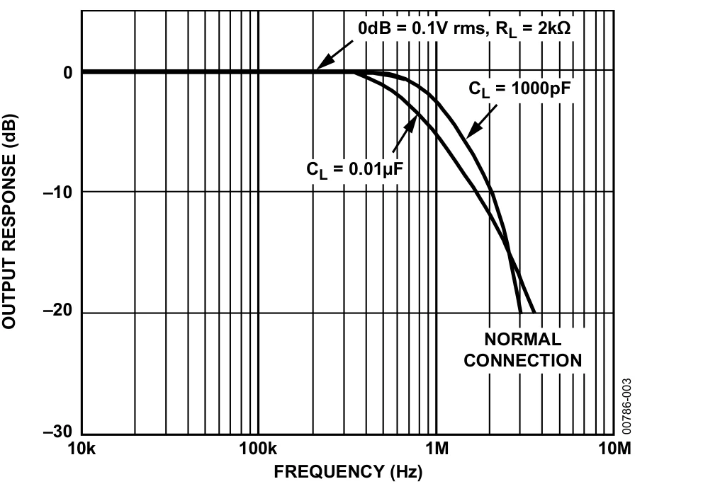
6.5 Bandwidth: mix at audio frequencies
= 1 V at 6 kHz, = 1 V at 5 kHz, = 0. Equations (2) and (6) give
Each line is only 50 mV, because of the 10 V divisor, and both lie far inside the bandwidth. Radio-frequency examples such as 10.7 MHz and 10.0 MHz are fine for an ideal mixer but past the AD633's corner; that is a job for the NE602.
7 Squaring
7.1 Tie X to Y
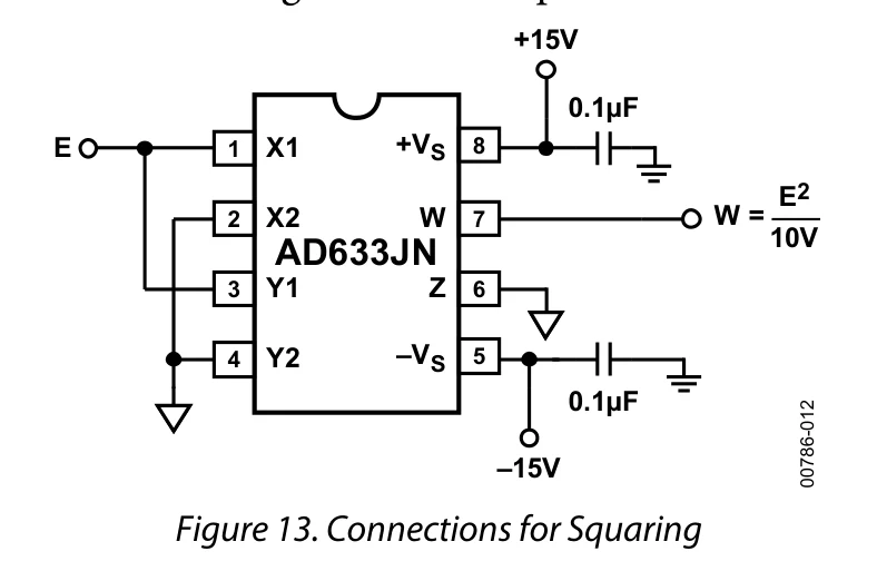
With and , Equation (6) becomes
The output is positive whichever sign the input has, so the squarer throws the sign away. That makes a quick first test of your wiring: +4 V and −4 V in should both give about +1.6 V out.
7.2 Predict before you measure
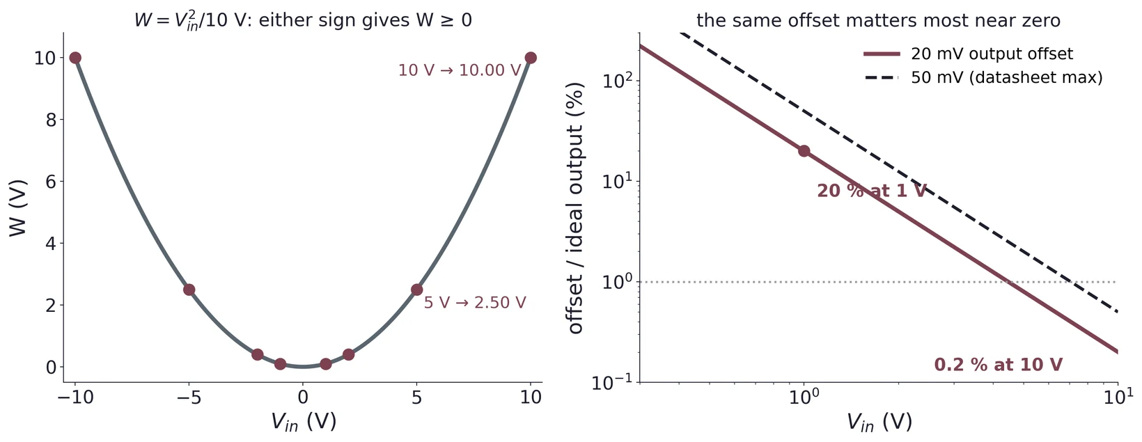
| ±1 V | ±2 V | ±5 V | ±10 V | |
|---|---|---|---|---|
| 0.10 V | 0.40 V | 2.50 V | 10.0 V |
Note how small the output is near zero: 100 mV at 1 V in. A 20 mV offset is then a 20 % error. This is why the offset work in Task 2 matters, and why Task 3 insists on offsets under ±50 mV before the square root. Take points on both sides of zero and more of them near zero, where the curve is flat and the errors are proportionally largest.
7.3 A sine in, twice the frequency out
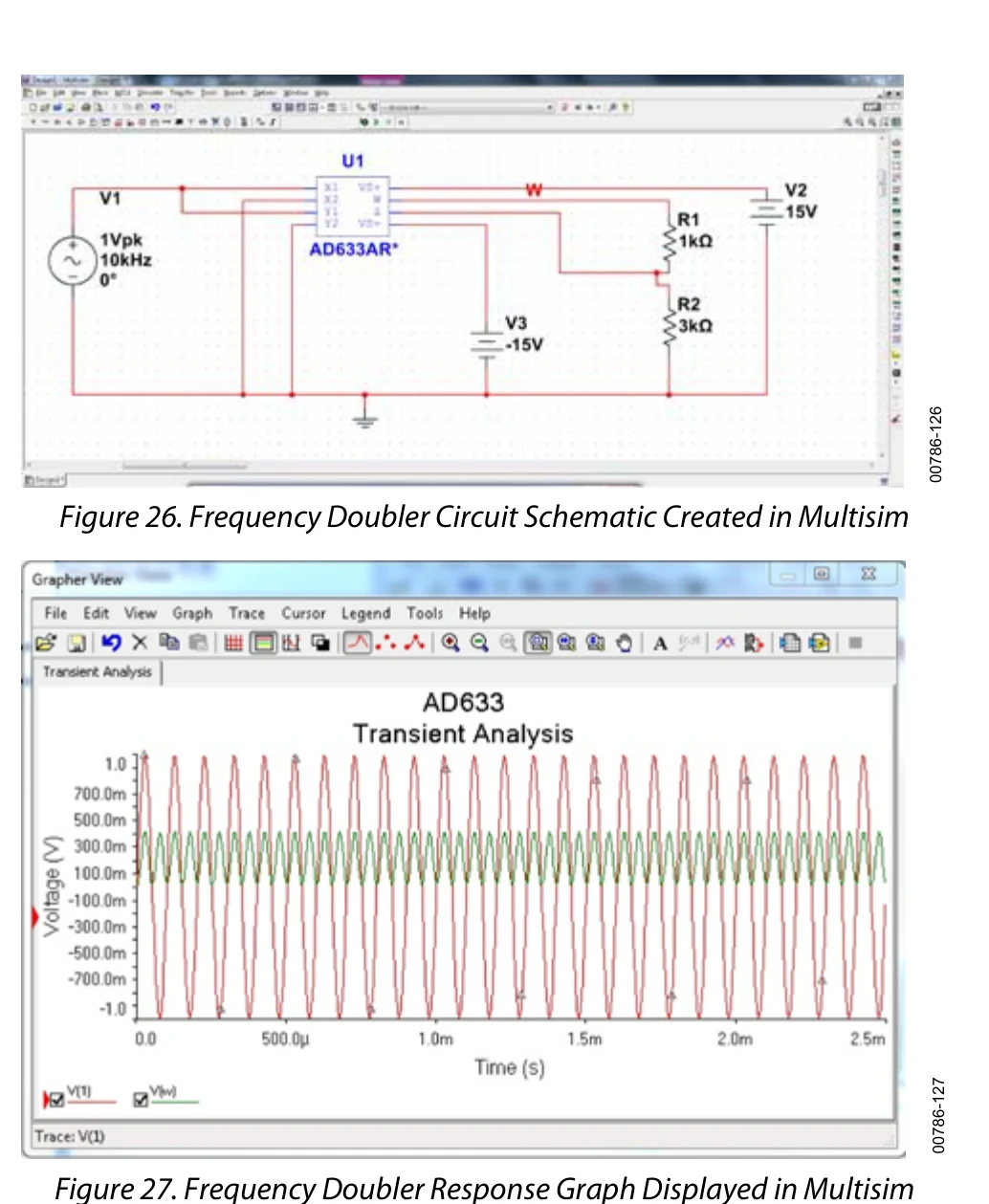
With , Equation (2) with equal frequencies gives
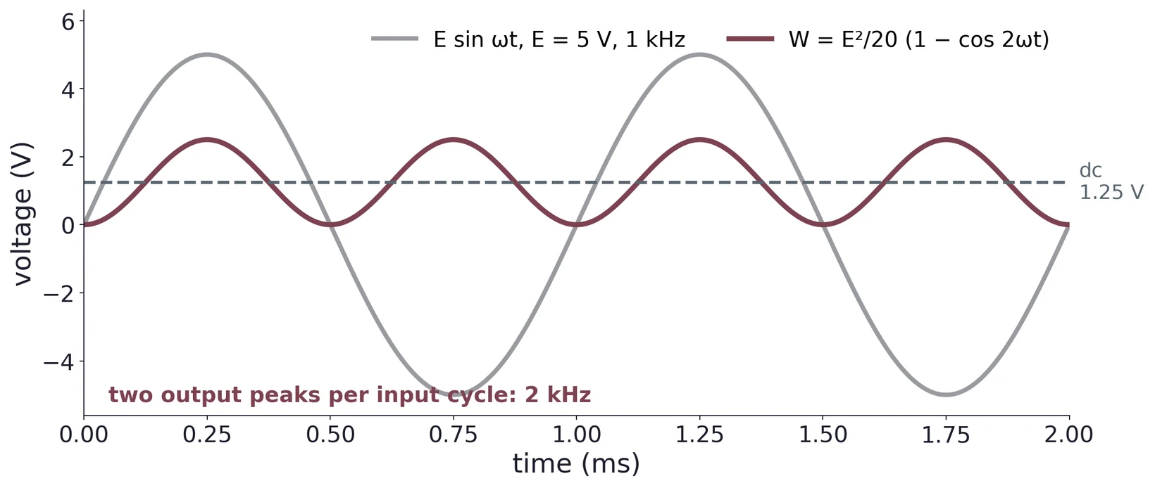
On the scope, a doubled frequency and a trace that never goes negative confirm the squarer works. The datasheet shows the same idea as a SPICE simulation (drawn in Multisim):
7.4 Fitting the data
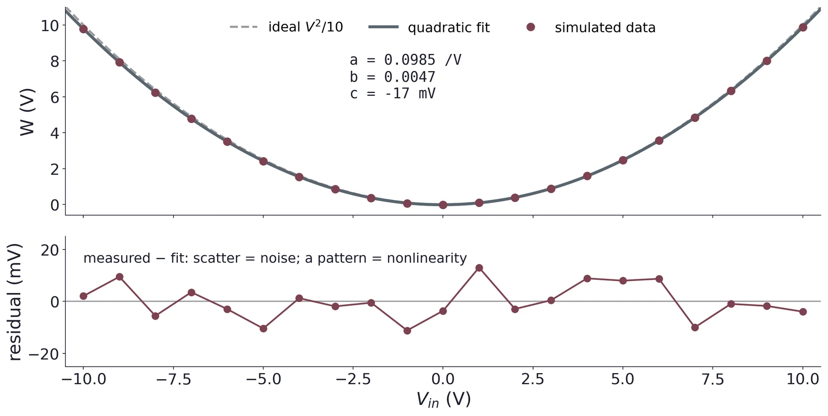
Task 1 asks for a quadratic fit with your Python code and plot. Fit the general form rather than forcing it through the origin:
| Call | What it gives you |
|---|---|
numpy.polyfit(v, w, 2) | The coefficients , , of a least-squares quadratic, highest power first |
numpy.polyval(p, v) | The fitted curve at the points v, for plotting and for residuals |
scipy.optimize.curve_fit(f, v, w) | A fit of any model function f, with a covariance matrix for uncertainties |
Each coefficient means something physical, and explaining what each one tells you about the chip is the heart of the task (§8.2).
8 Error Sources and Offset Trimming
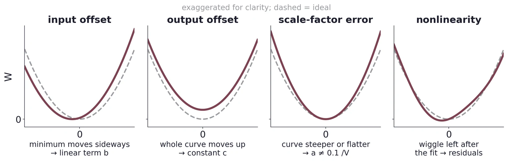
8.1 Four errors, four signatures
| Error | What it is | Signature in a squaring measurement | Fix |
|---|---|---|---|
| Input offset | A small unwanted voltage added at X or Y | Linear term ; the minimum sits away from = 0 | Trim network on or |
| Output offset | A fixed voltage added to | Constant ; the output is not zero for zero input | Trim network on |
| Scale-factor error | The divisor is not exactly 10 V | differs from 0.100 V⁻¹; error grows with the output | Cannot be trimmed with the offset network; measure and report it |
| Nonlinearity | What remains after the above are removed | A pattern in the fit residuals, not scatter | None; it is the device's floor (0.1–0.4 % of full scale) |
8.2 What the fit coefficients mean
Model the squarer with a single input offset and an output offset . (Strictly, X and Y each have their own offset, and ; tying the inputs together does not make those equal. The fit measures their average, , and the difference changes the constant term by a negligible .)
Matching Equation (9) term by term gives
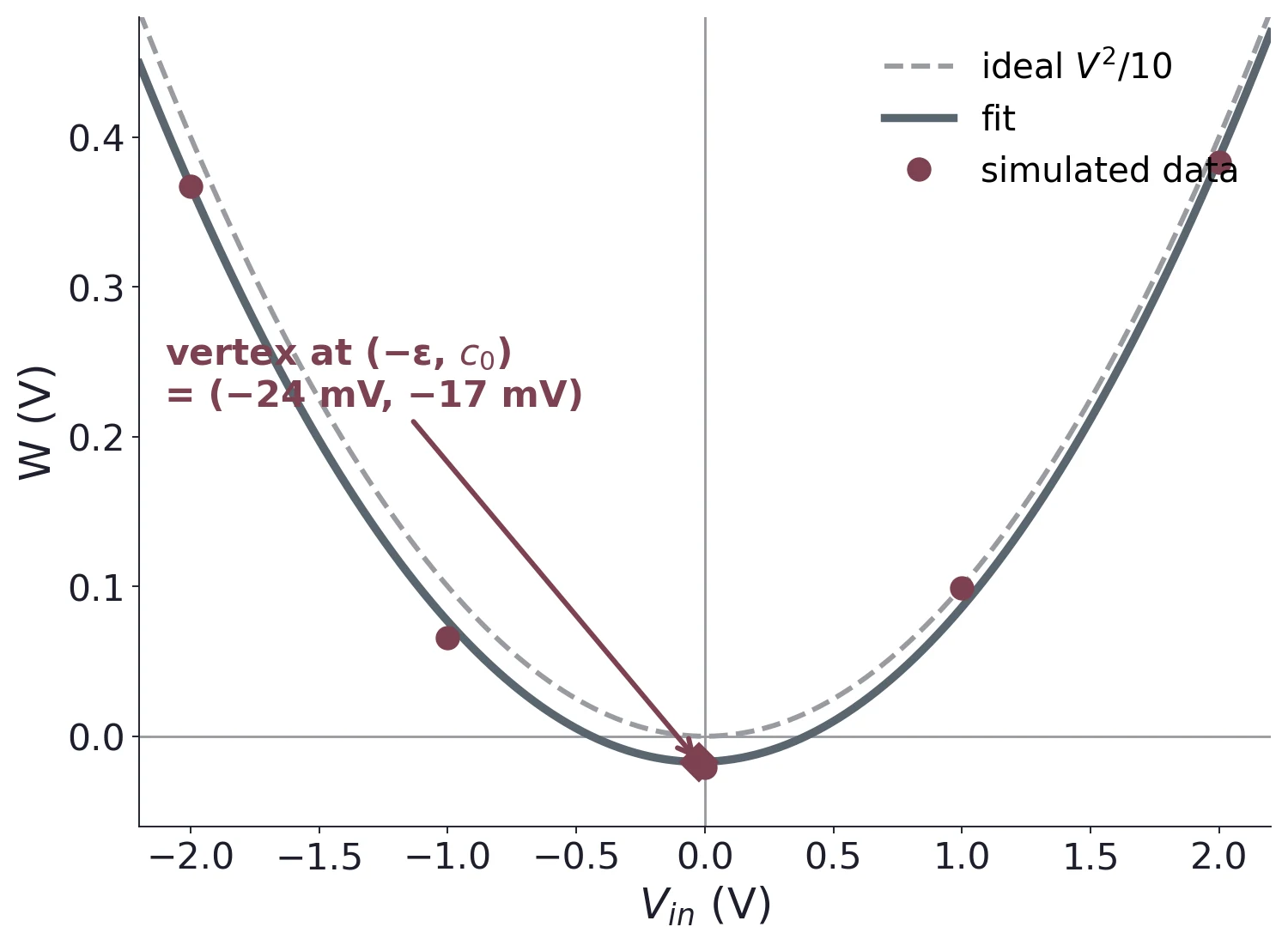
= 0.0985 V⁻¹, = 0.0047, = −17.0 mV.
- Scale error: %.
- Input offset: mV. That is inside the datasheet's ±30 mV maximum and the ±50 mV Task 3 allows, but it is still worth trimming. At 1 V in, the linear term adds 4.7 mV to an output of only 98.5 mV, an error of about 5 %.
- Output offset: mV.
Report all three with units and say what each one tells you about the device. If a fit ever gives an offset beyond the datasheet maximum, suspect the setup before the chip: a supply or signal generator that is not really at 0 V, or an input left floating.
8.3 Plot the residuals
On a plot of the raw data a good fit and a mediocre one look identical, because the quadratic dominates. Plot the residuals, measured minus fitted. A free quadratic fit absorbs offsets into and , so its residuals test only what a quadratic cannot describe: noise and nonlinearity. Compare with the ideal separately when you want to show the scale and offset errors.
8.4 The datasheet trim network
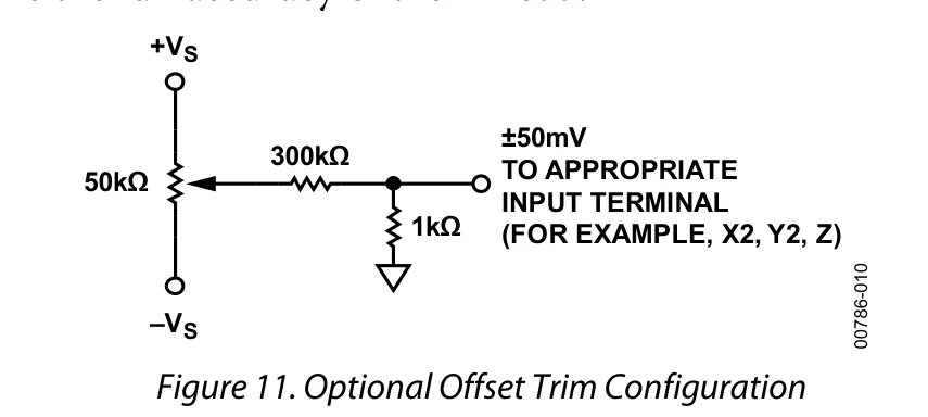
The pot swings its wiper anywhere from −15 to +15 V. The 300 kΩ and 1 kΩ divide that by 301, so the trim node covers
At the two ends of the pot's travel that range is exact. In between, the pot's own source resistance (at most 12.5 kΩ, at mid travel) adds to the 300 kΩ and bends the knob-to-voltage relation by a few percent, which does not matter for a trim. The 1 kΩ keeps the trimmed input close to ground, so the network adds only a small, adjustable voltage where the grounded return would otherwise be. The datasheet: "the input and output offsets can be eliminated by using the optional trim"; scale-factor error and nonlinearity remain.
8.5 Trim in order
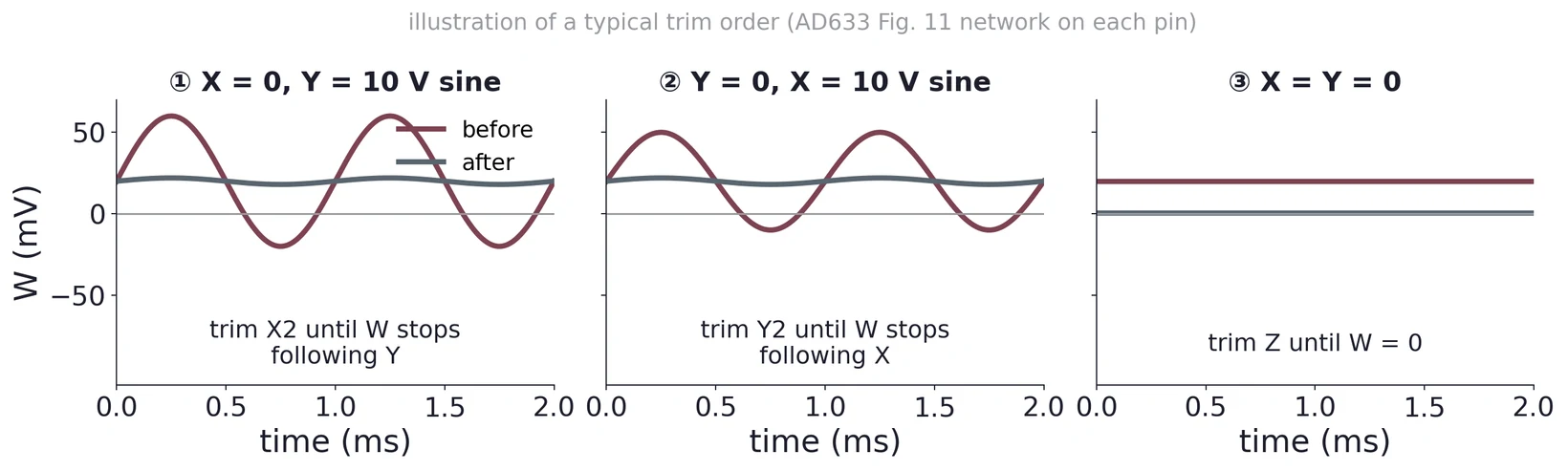
The order follows from Equation (6) with offsets included: . With = 0 the output contains , which follows ; nulling that removes alone. Swapping the roles removes . Only then does the zero-input output equal , which the trim cancels. If you trim first, the output reads zero at zero input while the input offsets are still there, and the error comes back as soon as you apply a signal.
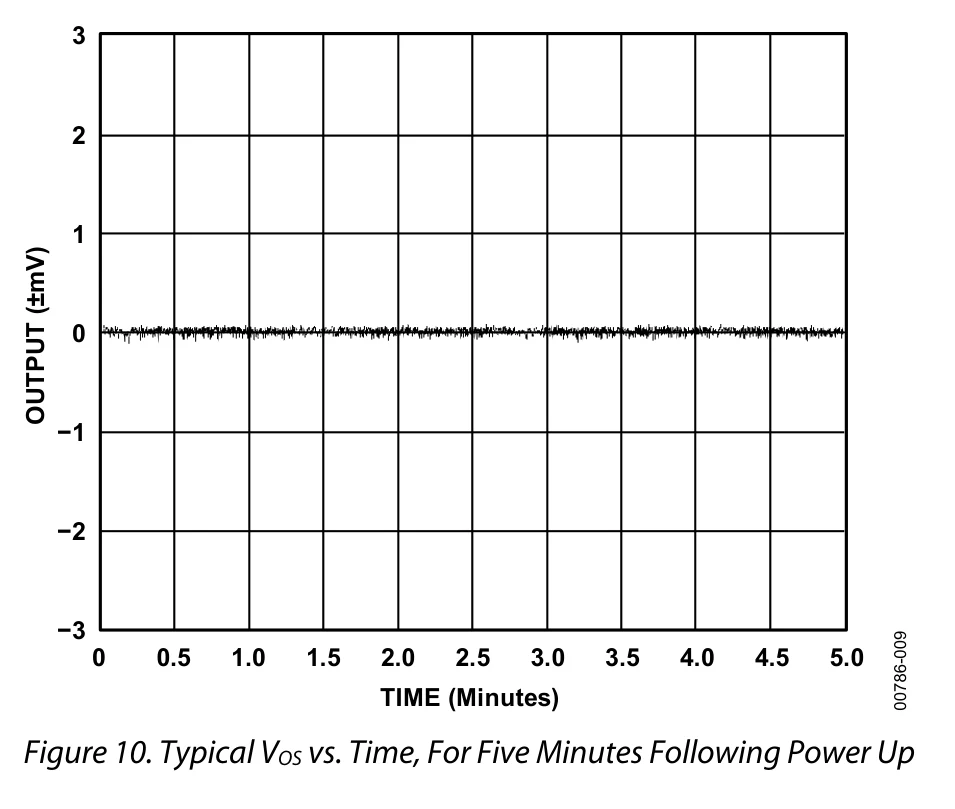
Draw the trim circuit with values and say which pin each network drives. Report the offsets numerically before and after trimming, and confirm they are within ±50 mV before starting Task 3. Then show the residual plot and quote the scale-factor error, which trimming cannot remove.
(a) A quadratic fit returns = 0.1030 V⁻¹, = −0.0082, = 24 mV. Find the scale-factor error, and .
(b) With those coefficients, what output would you measure at = 0, and what is the percentage error at = 2 V?
(c) Redesign the trim network for a ±20 mV range from the same ±15 V pot. Which resistor changes?
9 The Square Root by Feedback
9.1 Feedback inverts a function
Place a block that computes in the feedback path of a high-gain amplifier, and the closed loop computes . The loop drives its output to whatever value makes the fed-back quantity match the input. This works over any range where only rises (or only falls); elsewhere the inverse is not unique, and the loop needs help, like the diode in §9.2. If the feedback block squares, the loop must be delivering a square root. The same idea makes a logarithmic amplifier from a diode's exponential law.
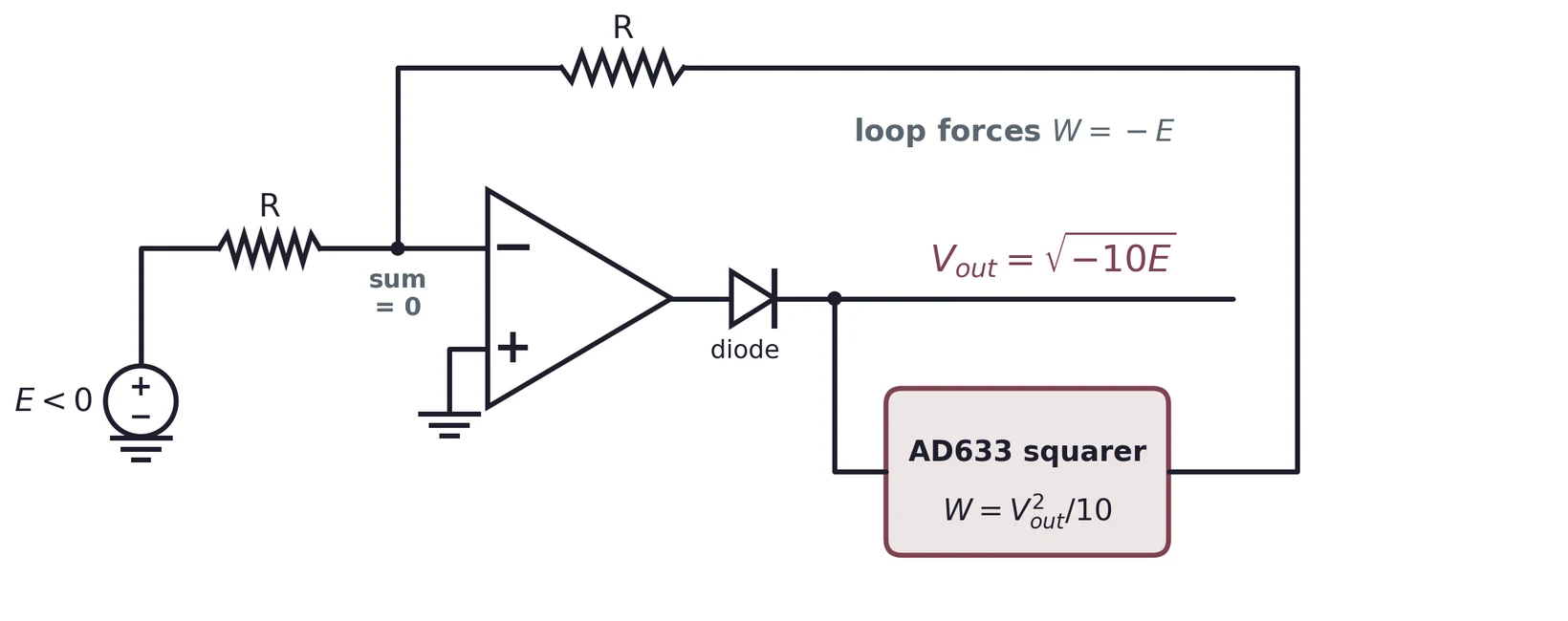
The summing node is a virtual ground, so the two currents into it must cancel: , or . The squarer sets , so
9.2 The datasheet circuit
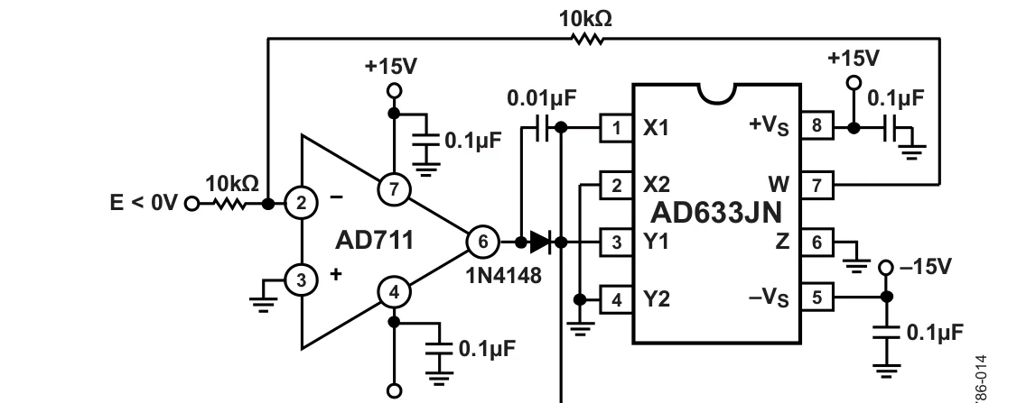
The datasheet uses an AD711 op-amp; a general-purpose op-amp such as the LM741 should serve at the slow, near-DC inputs of Task 3. The 1N4148 matters: "the diode is required to prevent latchup, which can occur … if the input were to change polarity, even momentarily." If goes positive, no real satisfies Equation (13). Without the diode, the op-amp then drives its output toward the negative rail. But the square of a large negative voltage is large and positive, so the fed-back current pushes the op-amp further the same way, and the loop can stay stuck there even after goes negative again. That is latchup. The diode blocks negative outputs, so the loop can only run with .
9.3 Where the square root struggles
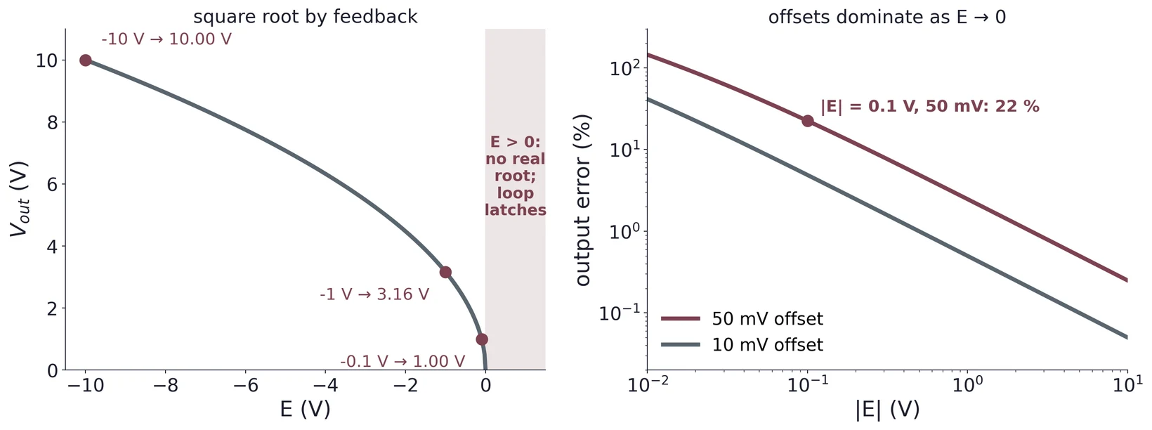
Two effects spoil the low end. First, the loop gain: a small change changes by , so the feedback fraction, and with it the loop's ability to correct errors, is proportional to and vanishes at zero. Second, offsets: an offset of size at the input shifts by , up or down depending on its sign. In the bad direction, , which is , 22 % high, for = 50 mV and = 0.1 V. Expect the square-root fit to be worst at the low end, and say so.
For the Task 3 fit, fit (or ) rather than forcing , and compare the fitted with the ideal .
(a) Predict for = −0.4, −2.5 and −6.4 V.
(b) Your offsets are trimmed to ±10 mV. Below what does the offset alone cause more than 5 % error?
(c) Explain why swapping the X inputs (so that ) lets the circuit accept positive instead. What else must change, and what is the sign of ?
10 Common Mistakes and Bench Safety
- Floating inputs. An unconnected X2, Y2 or Z has no path for its bias current and picks up noise, so the output wanders. Ground every unused input.
- Decoupling across the board. A capacitor 15 cm from the pin does little (§6.3). Put it at the pin.
- Wrong package map. The SOIC and PDIP pinouts differ. Check the marking.
- Trimming in the wrong order. Trimming Z first hides the input offsets (§8.5).
- Positive input to the square-root loop. It latches without the diode, and has no answer with it. Keep negative, and start from a few volts, not from zero.
- Reading near zero only. Offsets dominate there. Take points across the whole ±10 V range, with extra points near zero.
11 Self-Check
- What frequencies result when 5.0 kHz and 4.3 kHz are multiplied, and which circuit element selects one of them?
- Why does a single diode produce many more frequencies than a multiplier does?
- A receiver has = 455 kHz and = 1355 kHz with high-side injection. Which station is received, and where is the image?
- What does the Gilbert cell in the NE602 do with its oscillator input?
- For the AD633 with = 0 and both inputs tied to 3.0 V, what is ? What if both are tied to −3.0 V?
- Why must each 0.1 µF decoupling capacitor sit at its supply pin?
- In a quadratic fit to squaring data, what does a non-zero linear coefficient tell you, and how do you correct it in hardware?
- How does the datasheet trim network produce ±50 mV from a ±15 V pot?
- Why does a squarer in a feedback loop produce a square root, and what is the diode for?
- Why is the square root least accurate near zero input?
12 Practical Engineering Connections
- Frequency mixers. Radio receivers and transmitters, software-defined radios, radar and spectrum analyzers all mix signals to move information to a frequency that is easier to filter and amplify.
- Integrated mixers. NE602/SA602-style ICs combine an oscillator and a Gilbert-cell mixer in low-power receiver front ends for shortwave, amateur and communications equipment.
- Analog multipliers. The AD633 supports amplitude modulation, synchronous and phase-sensitive detection (the lock-in amplifier), voltage-controlled gain and filters, and true-RMS and power measurement: power is the product of voltage and current.
- Function inversion by feedback. The square-root loop is the same principle behind log and antilog amplifiers, dividers, automatic gain control and the linearization of nonlinear sensors.
- Calibration. Offset, scale and nonlinearity, measured by a fit and removed by a trim, are the error model of almost every sensor and converter in this course, including the ADC of Lab 8.