Part 1 · A mixer moves a signal to a new frequency
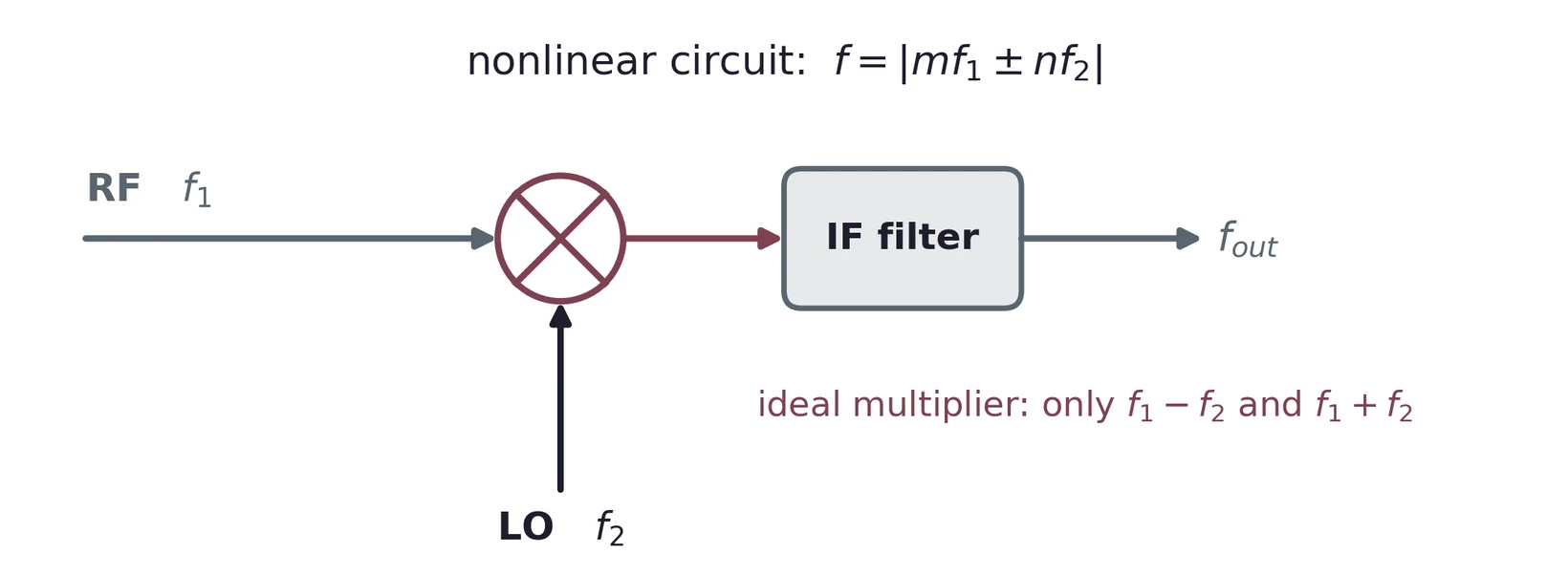
RF in, local oscillator (LO) in, a filter picks the output. The AD633 in Lab 2 is a precise mixer for about $20: it multiplies two voltages.
In time: a beat at the difference frequency
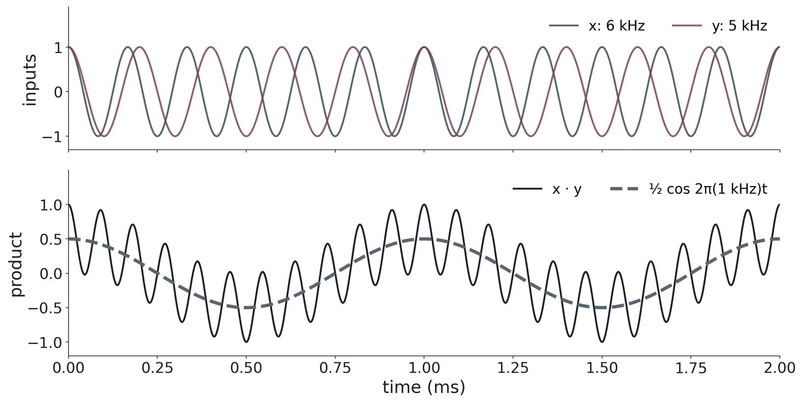
The product wobbles at 11 kHz inside a 1 kHz envelope. A low-pass filter keeps the dashed 1 kHz term; a band-pass at 11 kHz keeps the sum.
In frequency: two new lines, and a 6 dB loss
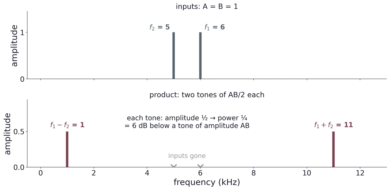
Each tone has amplitude . Power goes as , so each carries ¼ of the power of a tone of amplitude : 6 dB down. Keeping one throws the other away.
Any nonlinear circuit mixes
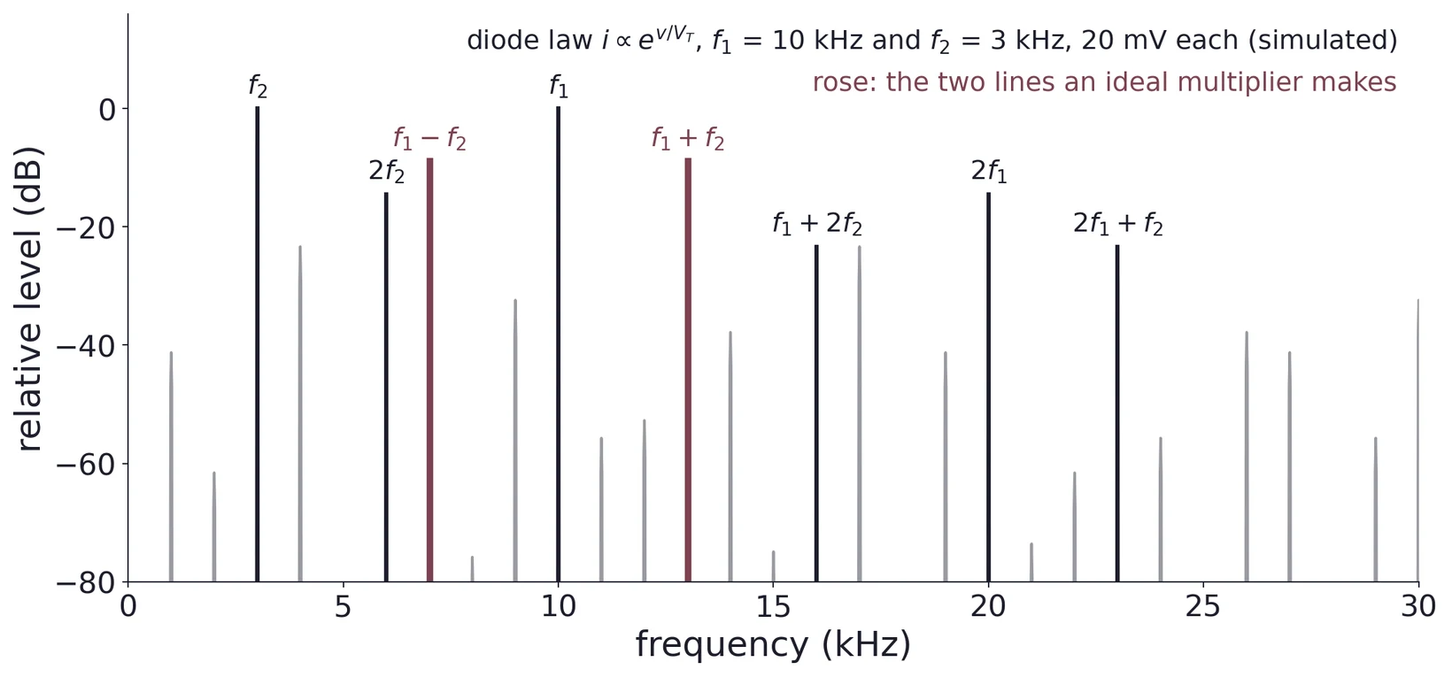
A diode's exponential law makes every , not just the two products. A multiplier makes only ; a real mixer relies on the filter after it.
Part 2 · The superheterodyne receiver
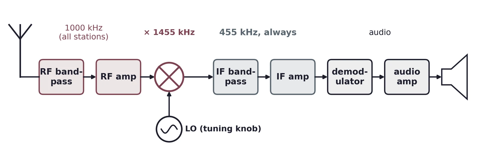
Tuning moves only the LO. Whichever station you tune lands on the same intermediate frequency (IF), where one fixed, sharp filter and amplifier do the work: 455 kHz for AM, 10.7 MHz for FM.
The image: a second station that also lands on the IF
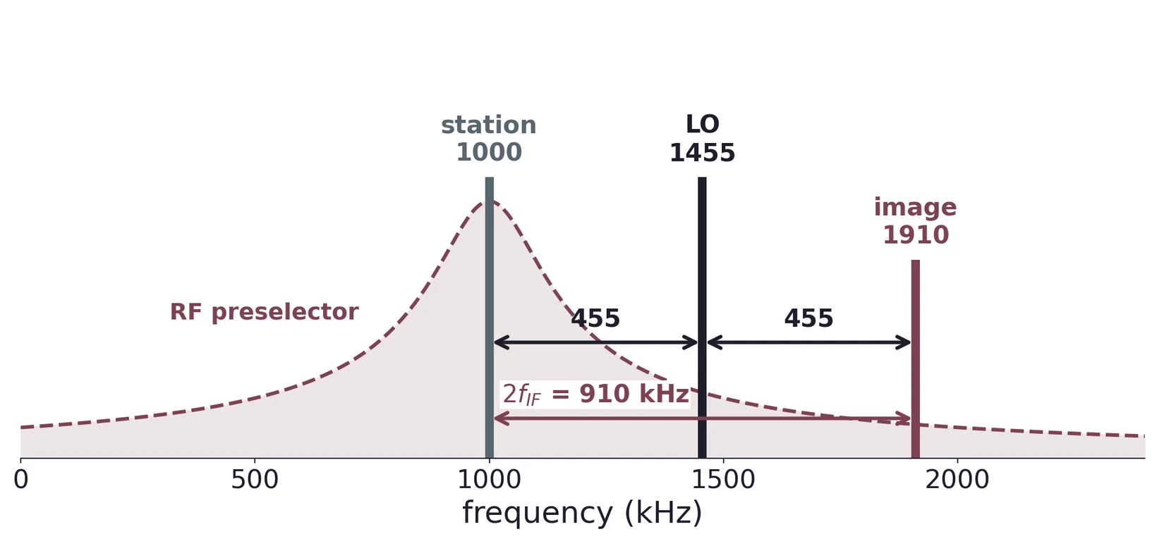
= 1455 kHz. The mixer only sees , so 1910 kHz gives 455 kHz too. The RF filter must reject it, away.
The mixer carries AM or FM along unchanged
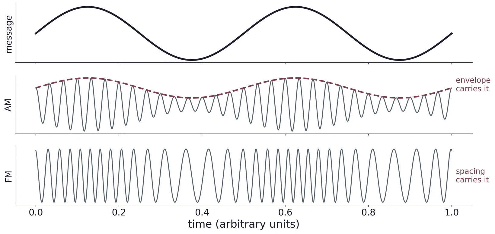
Shifting a carrier in frequency keeps its envelope (AM) and its frequency swings (FM). Only the demodulator after the IF knows the difference.
NE602 (SA602A): mixer and oscillator in one chip
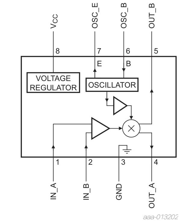
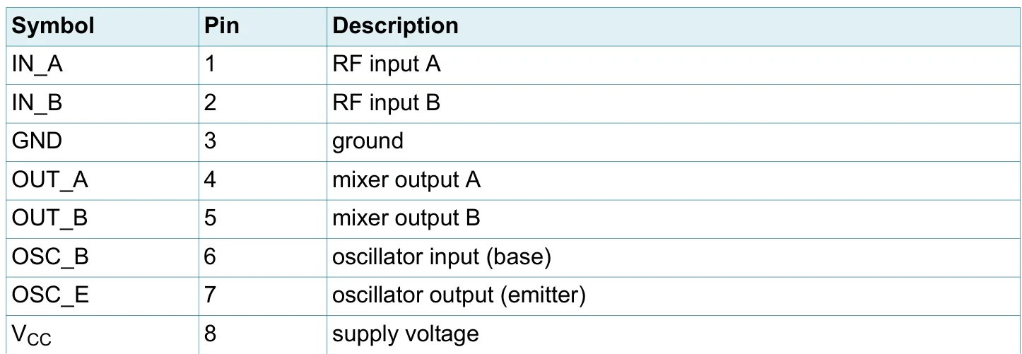
RF in on pins 1–2, oscillator on 6–7, mixer out on 4–5, supply 4.5–8 V on pin 8.
NXP SA602A Rev. 3, Fig. 1 and Table 3. Inputs to 500 MHz, oscillator to 200 MHz.
Inside the NE602: a Gilbert cell
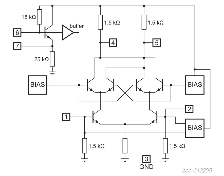
RF (pins 1, 2) drives a differential pair.
The oscillator switches the upper cross-coupled pairs.
Output current ≈ RF × sign(LO): a switching multiplier.
17 dB conversion gain at 45 MHz.
Part 3 · Inside the AD633
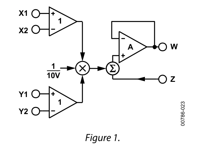
Differential X and Y inputs.
A buried Zener sets the 10 V scale.
adds after the product.
AD633JN pinout
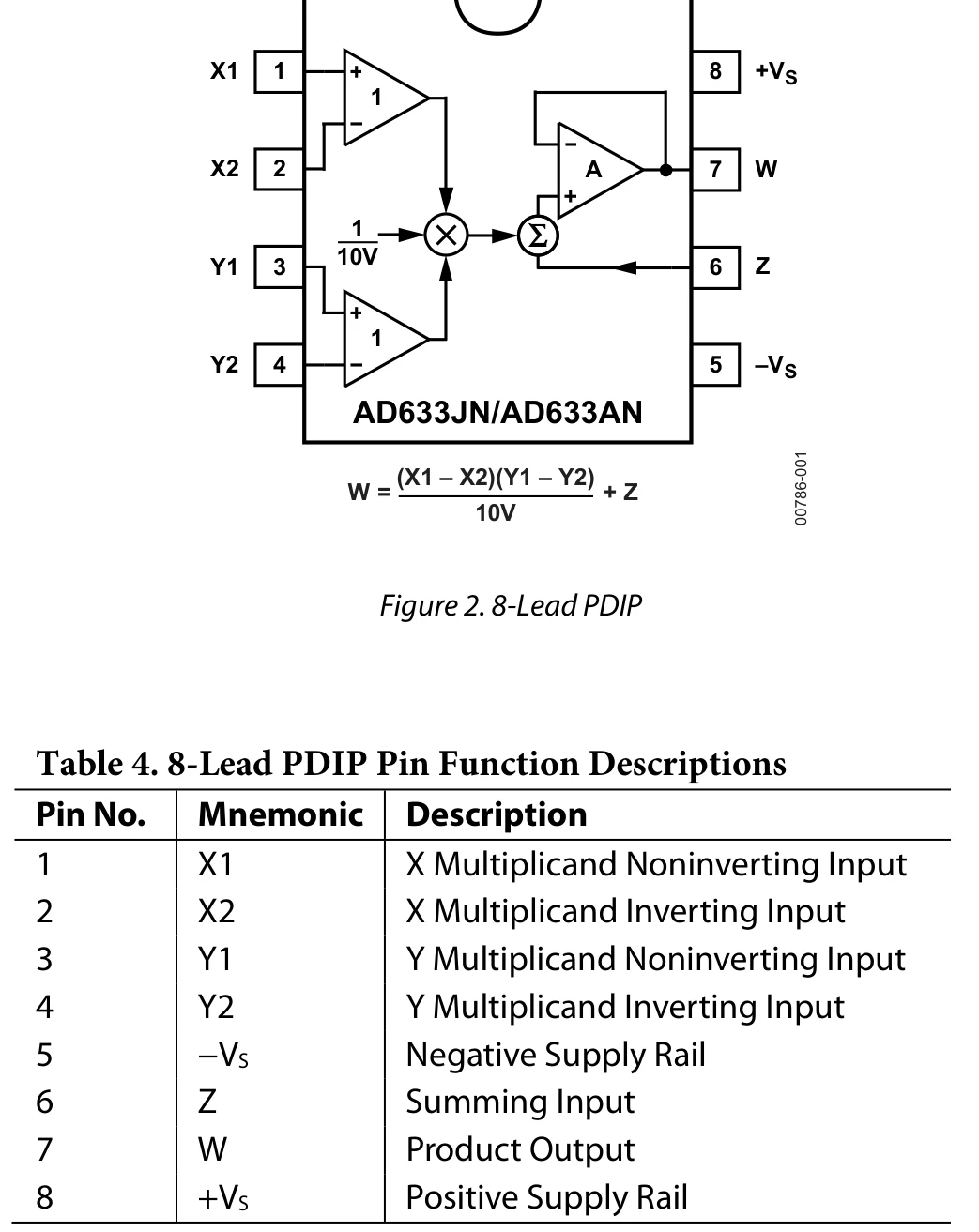
Pins 1, 2: ,
Pins 3, 4: ,
Pin 5: −15 V, pin 8: +15 V
Pin 6: , pin 7:
The SOIC version (AD633JR) is wired differently: check the marking.
Lab 2 wiring: returns grounded, rails decoupled
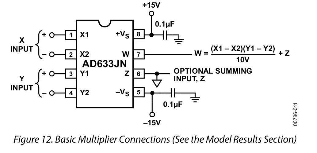
, and go to ground, never left floating. A 0.1 µF capacitor from each rail to ground, at pins 8 and 5.
Why the 0.1 µF sits at the pin
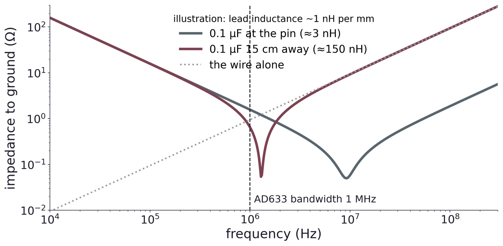
A capacitor is only a short to ground below its resonance. 15 cm of wire adds about 150 nH and moves that resonance near 1 MHz, right where the AD633 still has gain and can oscillate.
What the datasheet promises
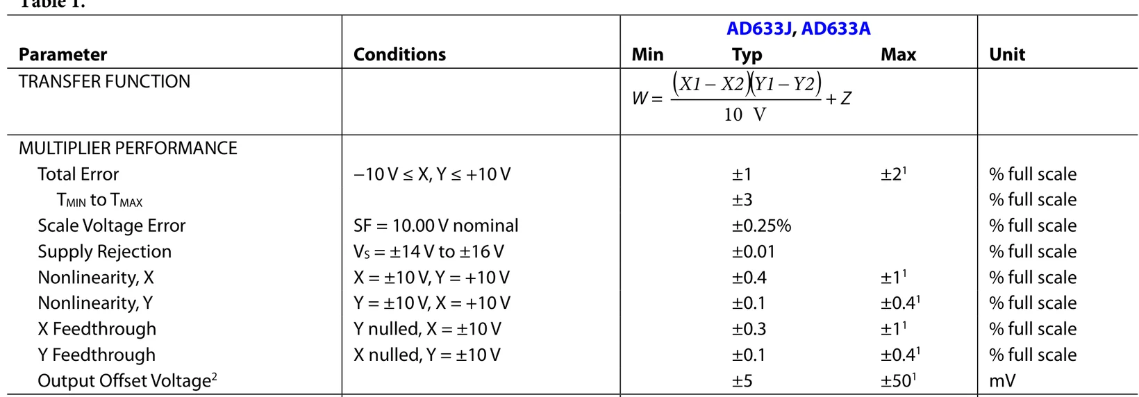
Total error ±2 % of full scale (10 V) at most. Output offset up to ±50 mV, input offset up to ±30 mV, scale error 0.25 %, nonlinearity 0.1–0.4 %. Lab 2 measures each one.
Bandwidth: 1 MHz, so mix in the audio range
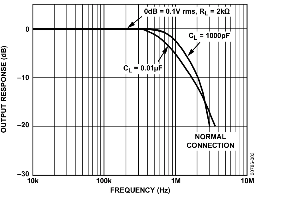
= 1 V at 6 kHz, = 1 V at 5 kHz, = 0:
Rev. K, Fig. 4. Two 1 V tones give only 50 mV lines; MHz radio signals are past the corner.
Part 4 · Tie X to Y: a squarer
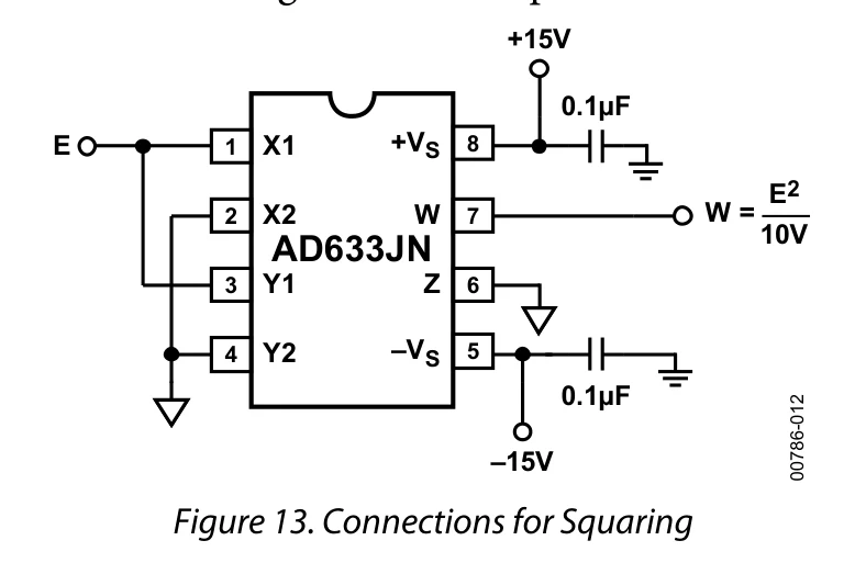
, :
Inverse:
Predict before you measure
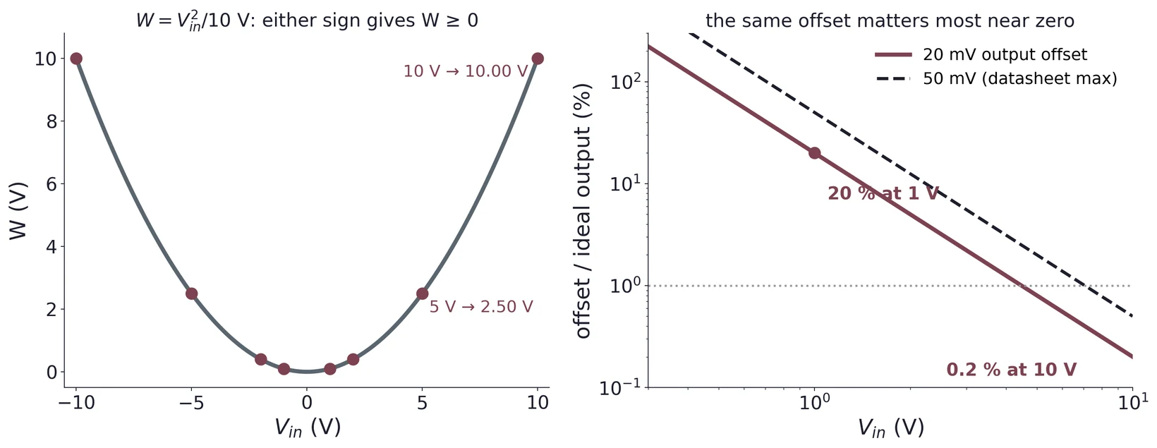
1 V → 0.10 V, 2 V → 0.40 V, 5 V → 2.50 V, 10 V → 10 V, for either sign. Near zero the output is tiny, so a 20 mV offset is already 20 % at 1 V.
A sine in, twice the frequency out
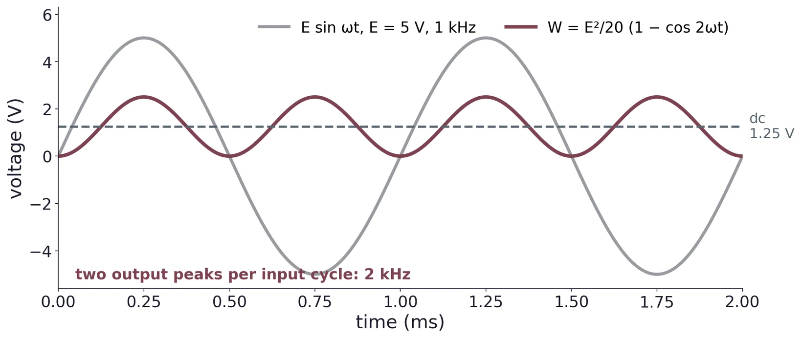
: a DC level plus a tone at . A quick scope test that the squarer works.
Fit a quadratic, then plot the residuals
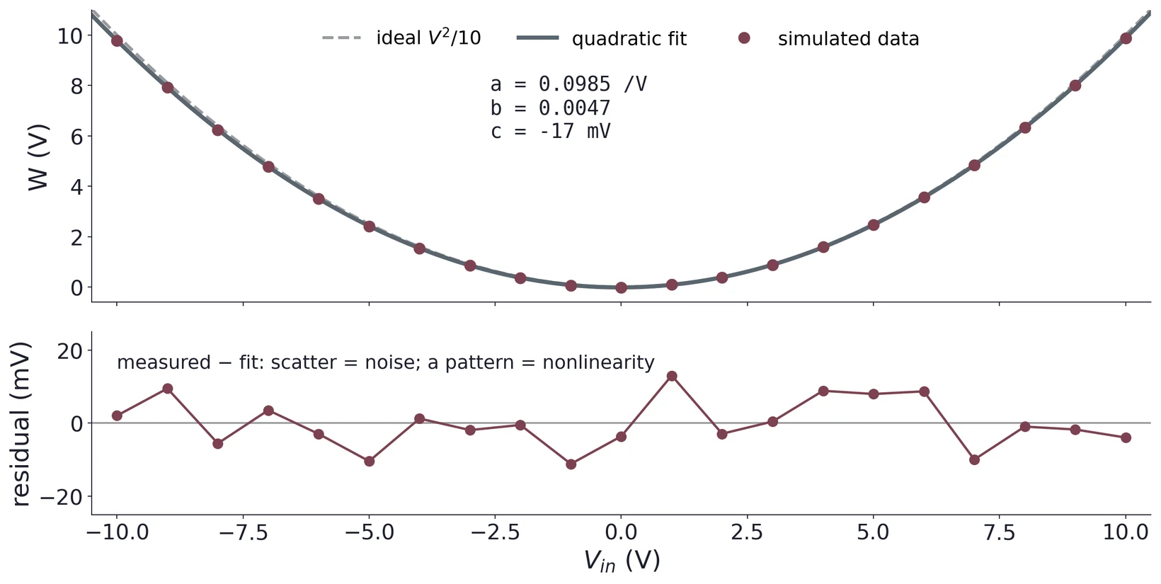
Simulated data. Fit (e.g. numpy.polyfit(v, w, 2)). On the curve a good and a poor fit look alike; the residuals show the difference.
Part 5 · Four errors, four signatures
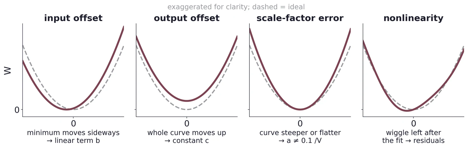
Datasheet: "input and output offsets can be eliminated by using the optional trim"; scale-factor error and nonlinearity cannot, so measure and report them.
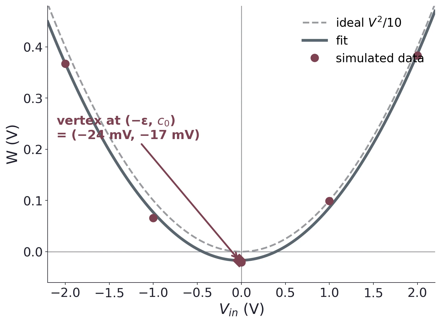
What the fit coefficients mean
So , .
| fit | means |
|---|---|
| a = 0.0985 /V | scale 1.5 % low |
| b = 0.0047 | ε = 24 mV |
| c = −17 mV | = −17 mV |
The datasheet trim network: ±50 mV
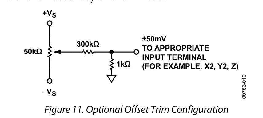
The pot swings from −15 V to +15 V.
300 kΩ and 1 kΩ divide it down:
One network per pin: , , .
Offsets trim out this way; scale error and nonlinearity do not (datasheet, Error Sources).
Trim in order: X, then Y, then Z
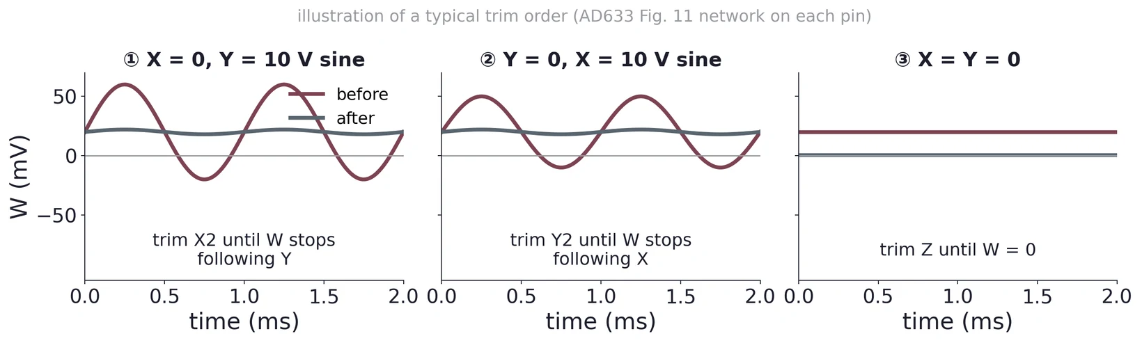
With X = 0, any output that follows Y is X's offset times Y: null it at . Swap for Y. Then, with both at zero, set at . Task 3 needs every offset under ±50 mV.
Part 6 · Feedback inverts a function
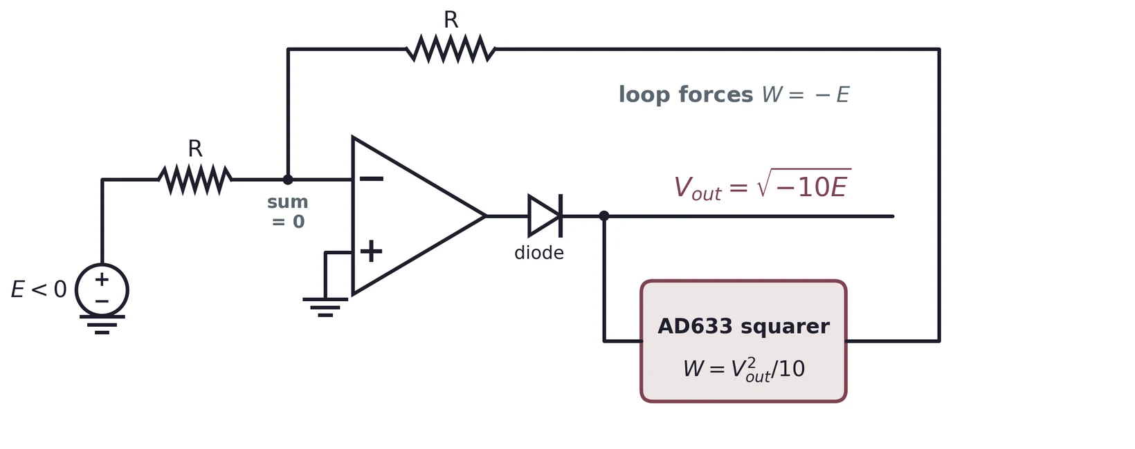
The summing node is at 0 V, so the currents and cancel: . The op-amp drives until , so .
The datasheet square-root circuit
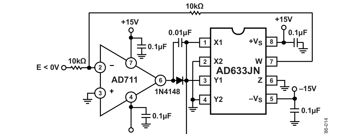
Rev. K, Fig. 15: output (after the diode) for . The 1N4148 blocks the wrong polarity; without it, a moment of latches the loop.
Where the square root struggles
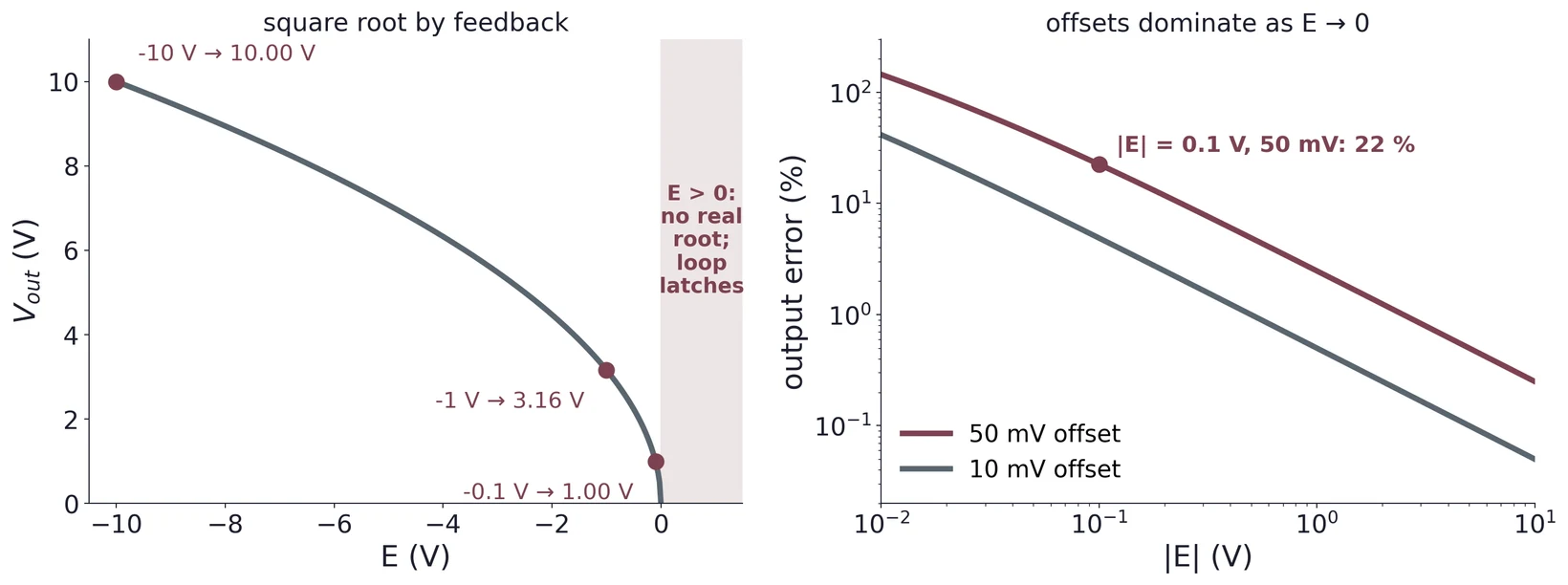
Near the square has no slope, so the loop gain collapses and any offset dominates: 50 mV is a 22 % error at = 0.1 V. Fit and expect the low end to fit worst.
Use ← → to move, Home / End to jump, and F for fullscreen.
Figure descriptions
Slide 2 · Part 1 · A mixer moves a signal to a new frequency
Mixer block diagram: the RF signal at f1 and the local oscillator at f2 enter a multiplier; its output passes an IF filter to give f_out. A general nonlinear circuit produces f = |m f1 ± n f2|; an ideal multiplier produces only f1 − f2 and f1 + f2.
Slide 4 · In time: a beat at the difference frequency
Top: two unit cosines at 6 kHz and 5 kHz over 2 ms. Bottom: their product oscillates rapidly inside an envelope, with the dashed difference term, one half cos 2π(1 kHz)t, tracing its slow 1 kHz component.
Slide 5 · In frequency: two new lines, and a 6 dB loss
Top: input spectrum with lines of amplitude 1 at f2 = 5 kHz and f1 = 6 kHz. Bottom: the product has lines of amplitude 0.5 at f1 − f2 = 1 kHz and f1 + f2 = 11 kHz, with the inputs gone; each tone has half the amplitude and a quarter of the power, 6 dB below a tone of amplitude AB.
Slide 6 · Any nonlinear circuit mixes
Simulated spectrum of a diode-law nonlinearity driven by 20 mV tones at f1 = 10 kHz and f2 = 3 kHz: besides the inputs, many products appear at 2f2, f1 − f2, f1 + f2, f1 + 2f2, 2f1, 2f1 + f2 and others; the two lines an ideal multiplier would make, 7 and 13 kHz, are highlighted.
Slide 7 · Part 2 · The superheterodyne receiver
Superheterodyne receiver: antenna, RF band-pass, RF amplifier, mixer driven by a tunable local oscillator, IF band-pass, IF amplifier, demodulator, audio amplifier, speaker. Example: all stations near 1000 kHz, times 1455 kHz from the oscillator, give 455 kHz at the IF, always.
Slide 8 · The image: a second station that also lands on the IF
Frequency axis from 0 to 2400 kHz: the wanted station at 1000 kHz inside the RF preselector's passband, the LO at 1455 kHz 455 kHz above it, and the image at 1910 kHz a further 455 kHz above; station and image are 2 f_IF = 910 kHz apart, and the preselector is far down at the image.
Slide 9 · The mixer carries AM or FM along unchanged
A slow sine message; an AM signal whose envelope follows the message; an FM signal of constant amplitude whose cycles bunch and spread with the message.
Slide 10 · NE602 (SA602A): mixer and oscillator in one chip
NXP SA602A datasheet Fig. 1, block diagram: a voltage regulator on pin 8 VCC; an oscillator on pins 7 (emitter) and 6 (base) whose buffered output drives a multiplier; an input amplifier from pins 1 and 2 (IN_A, IN_B) feeding the multiplier; mixer outputs on pins 4 and 5; ground on pin 3.
NXP SA602A datasheet Table 3, pin description: IN_A pin 1 RF input A; IN_B pin 2 RF input B; GND pin 3 ground; OUT_A pin 4 mixer output A; OUT_B pin 5 mixer output B; OSC_B pin 6 oscillator input (base); OSC_E pin 7 oscillator output (emitter); VCC pin 8 supply voltage.
Slide 11 · Inside the NE602: a Gilbert cell
NXP SA602A datasheet Fig. 3, equivalent circuit: a Gilbert cell. A lower differential transistor pair driven from pins 1 and 2 with 1.5 kΩ emitter resistors feeds two cross-coupled upper pairs switched by the buffered oscillator from pins 6 and 7; 1.5 kΩ collector loads connect to outputs 4 and 5; bias blocks set the operating currents.
Slide 12 · Part 3 · Inside the AD633
AD633 datasheet Rev. K Fig. 1, functional block diagram: inputs X1 and X2 feed one unity-gain differential amplifier and Y1 and Y2 another; their outputs are multiplied and scaled by 1/10 V, summed with the Z input, and buffered by amplifier A to output W.
Slide 13 · AD633JN pinout
AD633 datasheet Rev. K Fig. 2 and Table 4, 8-lead PDIP AD633JN/AN: pin 1 X1, 2 X2, 3 Y1, 4 Y2, 5 minus VS, 6 Z summing input, 7 W product output, 8 plus VS, with W = (X1 − X2)(Y1 − Y2)/10 V + Z.
Slide 14 · Lab 2 wiring: returns grounded, rails decoupled
AD633 datasheet Rev. K Fig. 12, basic multiplier connections: X input across pins 1 and 2, Y input across pins 3 and 4, pin 8 to +15 V and pin 5 to −15 V each with a 0.1 µF capacitor to ground, pin 6 as the optional summing input Z, and output W = (X1 − X2)(Y1 − Y2)/10 V + Z on pin 7.
Slide 15 · Why the 0.1 µF sits at the pin
Illustration of impedance to ground against frequency for a 0.1 µF capacitor: at the pin with about 3 nH it stays low to about 10 MHz, dipping at its resonance; 15 cm away with about 150 nH it resonates near 1.3 MHz and rises along the wire's own reactance above that; a line marks the AD633's 1 MHz bandwidth.
Slide 16 · What the datasheet promises
AD633 datasheet Rev. K Table 1, multiplier performance at 25 °C and ±15 V: total error ±1 % typical, ±2 % maximum of full scale for inputs within ±10 V; scale voltage error ±0.25 %; supply rejection ±0.01 %; nonlinearity X ±0.4 % typical, ±1 % maximum, Y ±0.1 % typical, ±0.4 % maximum; X and Y feedthrough; output offset voltage ±5 mV typical, ±50 mV maximum.
Slide 17 · Bandwidth: 1 MHz, so mix in the audio range
AD633 datasheet Rev. K Fig. 4, frequency response: output flat at 0 dB from 10 kHz to about 300 kHz, then falling, about −3 dB near 1 MHz and −20 dB near 3 MHz, with curves for 0.01 µF and 1000 pF loads.
Slide 18 · Part 4 · Tie X to Y: a squarer
AD633 datasheet Rev. K Fig. 13, connections for squaring: input E drives both X1 and Y1, X2, Y2 and Z are grounded, supplies ±15 V with 0.1 µF bypass capacitors, and the output is W = E²/10 V.
Slide 19 · Predict before you measure
Left: squarer output W = V_in²/10 V against V_in from −10 to 10 V, a parabola through 2.50 V at ±5 V and 10.00 V at ±10 V. Right: an output offset as a percentage of the ideal output against V_in on log axes: 20 mV is 20 % at 1 V and 0.2 % at 10 V; the 50 mV datasheet maximum is 2.5 times worse.
Slide 20 · A sine in, twice the frequency out
A 5 V, 1 kHz sine input and the squarer output W = E²/20 (1 − cos 2ωt) over 2 ms: the output stays between 0 and 2.5 V around a dashed dc level of 1.25 V and peaks twice per input cycle, at 2 kHz.
Slide 21 · Fit a quadratic, then plot the residuals
Simulated squarer data from −10 to 10 V with the ideal V²/10 curve and a quadratic fit, a = 0.0985 per volt, b = 0.0047 and c = −17 mV. Below, the residuals, measured minus fit, scatter within about ±15 mV: scatter means noise, a pattern would mean nonlinearity.
Slide 22 · Part 5 · Four errors, four signatures
Four exaggerated squarer errors against the dashed ideal parabola: an input offset moves the minimum sideways, giving a linear fit term; an output offset lifts the whole curve, a constant; a scale-factor error makes the curve steeper; nonlinearity leaves a wiggle that shows in the residuals.
Slide 23 · What the fit coefficients mean
Zoom near zero of the simulated squarer fit: the fitted parabola sits below and slightly left of the dashed ideal V squared over 10, with data points at −2, −1, 0, 1 and 2 V. Its vertex is marked at minus epsilon and c0, about −24 mV and −17 mV.
Slide 24 · The datasheet trim network: ±50 mV
AD633 datasheet Rev. K Fig. 11, optional offset trim: a 50 kΩ potentiometer between plus VS and minus VS; its wiper feeds a 300 kΩ resistor to a node with 1 kΩ to ground, giving ±50 mV to the input terminal being trimmed, for example X2, Y2 or Z.
Slide 25 · Trim in order: X, then Y, then Z
Illustration of a typical trim order, output W in millivolts over 2 ms before and after: 1, with X = 0 and a 10 V sine on Y, trim X2 until W stops following Y; 2, with Y = 0 and a sine on X, trim Y2; 3, with X = Y = 0, trim Z until W = 0.
Slide 26 · Part 6 · Feedback inverts a function
Square root by feedback: a negative input E feeds the op-amp's inverting summing node through R; the op-amp output passes a diode to V_out, which drives an AD633 squarer giving W = V_out²/10; W returns through a second R to the summing node. The loop forces W = −E, so V_out = √(−10E).
Slide 27 · The datasheet square-root circuit
AD633 datasheet Rev. K Fig. 15, connections for square rooting: a negative input E drives the inverting input of an AD711 op-amp through 10 kΩ; the op-amp output passes through a 1N4148 diode to both X1 and Y1 of the AD633; the AD633 output W returns through 10 kΩ to the op-amp input; the output is W = square root of −(10 V)E.
Slide 28 · Where the square root struggles
Left: V_out = √(−10E) against E from −10 to 0 V, through 10.00 V at −10 V, 3.16 V at −1 V and 1.00 V at −0.1 V; for E above 0 there is no real root and the loop latches. Right: output error against |E| for 50 mV and 10 mV input offsets, rising as E approaches zero; a 50 mV offset gives 22 % error at |E| = 0.1 V.